What is Unsupervised Learning? Finding the Hidden Order in Chaos

In my previous post, we looked at Supervised Learning, where a machine learns from a teacher using labeled “flashcards.” It’s a structured, guided process where the right answer is always provided.

But what happens when there is no teacher? What happens when you have a mountain of data, but no labels, no categories, and no “correct answers” to guide the way?

Welcome to the world of Unsupervised Learning.

This is where AI acts more like an explorer than a student. It doesn’t wait to be told what is what; instead, it dives into the data to find the hidden structures and patterns that the human eye might miss.

The Non-Technical Explanation (The “Toy Box” Analogy)

Imagine you have a massive box of miscellaneous toys that has been dumped onto the floor. There are thousands of items: LEGO bricks of different colors, action figures, puzzle pieces, and toy cars.

You have no instructions. No one has told you “these are the blue ones” or “these are the vehicles.”

How would you make sense of this mess?

Even without a guide, your brain would naturally start to group things together based on their inherent characteristics:

1. By Color: You put all the red bricks in one pile and the blue ones in another.
2. By Shape: You put all the circular wheels together.
3. By Texture: You separate the soft plushies from the hard plastic toys.

This is Unsupervised Learning. The computer isn’t trying to “get the right answer” because there isn’t one defined yet. Instead, it is looking for similarities and differences. It identifies that “Data Point A” looks a lot like “Data Point B” but is nothing like “Data Point C.”

In the real world, this is how Netflix realizes that people who watch 80s synth-wave documentaries also tend to enjoy neon-noir sci-fi movies—even if no one has explicitly labeled those two genres as “connected.”

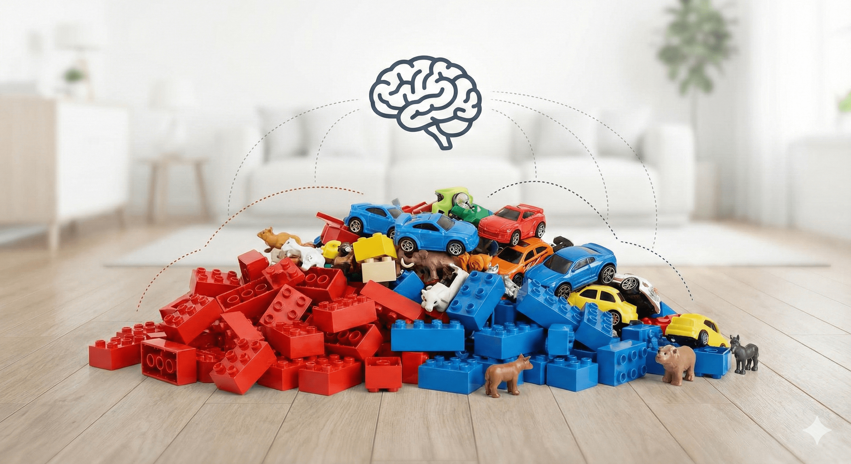
Figure: A visual analogy — grouping similar items from a messy collection.

The Technical Deep Dive

In technical terms, Unsupervised Learning is a type of machine learning that analyzes and clusters unlabeled datasets. These algorithms discover hidden patterns or data groupings without the need for human intervention.

The Core Difference: No $y$ Variable

Recall that in Supervised Learning, our goal was to find the mapping function $y = f(X)$.

In Unsupervised Learning, there is no $y$. We only have $X$ (the input features). The goal is to model the underlying structure or distribution in the data to learn more about it.

The Two Pillars of Unsupervised Learning

Most unsupervised tasks fall into two main categories:

1. Clustering (Grouping) This is the most common task. The goal is to find natural groupings in data. Points within a group (cluster) should be as similar as possible to each other and as different as possible from points in other groups.

• Real-world use: Customer segmentation for marketing (finding “high spenders” vs. “bargain hunters”).
• Image of Clustering:

2. Dimensionality Reduction (Simplifying) Sometimes, we have too much data—hundreds or thousands of features. This makes it hard for humans to visualize and hard for computers to process (a concept known as the “Curse of Dimensionality”). Dimensionality reduction squashes the data down to its most important parts without losing the core information.

• Real-world use: Compressing high-resolution images or simplifying genomic data.
• Image of Dimensionality Reduction:

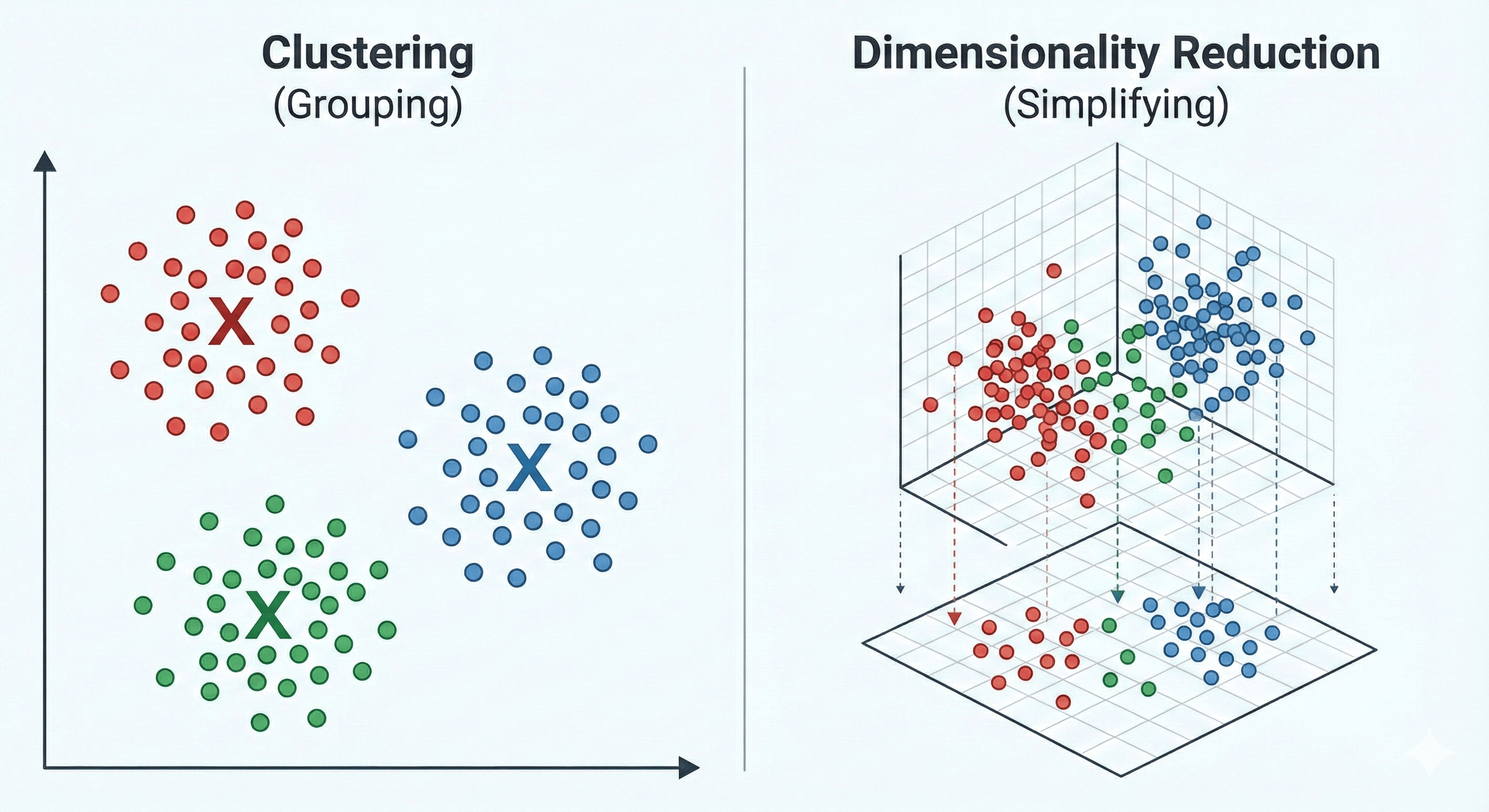
Figure: The two pillars of unsupervised learning — clustering and dimensionality reduction.

Why is it harder than Supervised Learning?

Unsupervised learning is often called “knowledge discovery.” It’s objectively harder because there is no ground truth to compare the results against.

If a supervised model predicts a house price, we can check the actual sale price. If an unsupervised model groups your customers into four segments, how do you know if “four” is the right number? Evaluation requires domain expertise and different mathematical metrics like the “Silhouette Score” or the “Elbow Method.”

The Coding Tutorial — Building a Clustering Model

We are going to build a K-Means Clustering model. This is the most famous unsupervised algorithm in existence.

The Scenario: Imagine we own a grocery store. We have a list of customers and we know two things about them:

1. Annual Income (in k$)
2. Spending Score (a score from 1-100 based on their behavior)

We want the AI to tell us how many natural “types” of shoppers we have, so we can tailor our marketing to them.

We will break this down into 5 parts:

1. Data Setup: Creating our unlabeled dataset.
2. The Elbow Method: Finding the “Optimal K” (How many clusters?).
3. Initialization & Training: Running the K-Means algorithm.
4. Visualization: Seeing the clusters the AI found.
5. Interpretation: Understanding what the clusters actually mean.

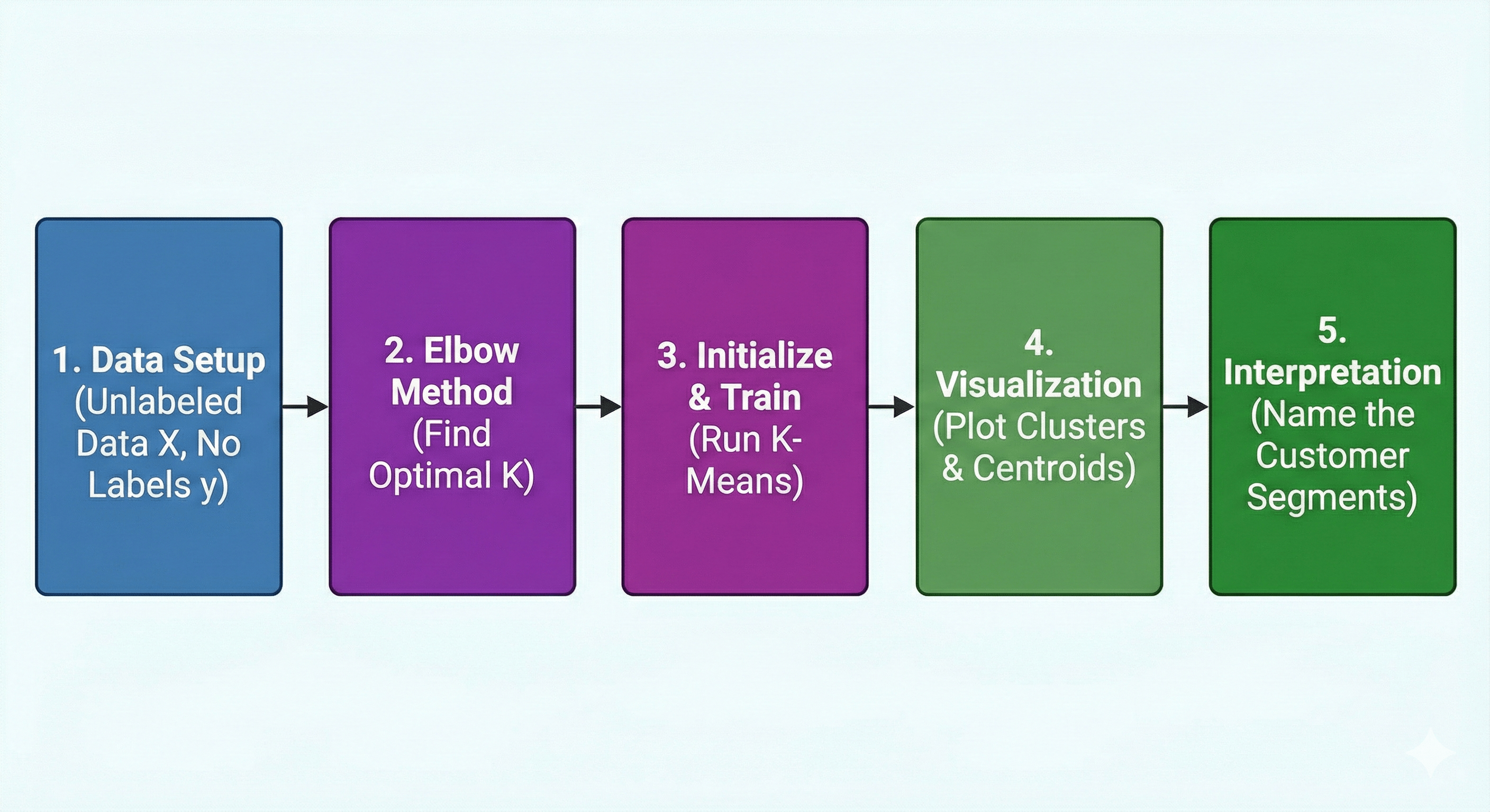
Figure: A high-level workflow showing the steps from raw data to cluster interpretation.

Step 1: Data Setup

import numpy as np
import pandas as pd
import matplotlib.pyplot as plt
from sklearn.cluster import KMeans

# --- STEP 1: Create Unlabeled Synthetic Data ---
# We are creating a dataset representing 100 grocery store customers.
# Unlike Supervised Learning, we do NOT provide any labels (no 'y').
# We only have Features: [Annual Income, Spending Score]

# Seed for reproducibility
np.random.seed(42)

# Generate synthetic data for 3 distinct types of shoppers:
# 1. Low Income, Low Spending
# 2. High Income, High Spending
# 3. Mid Income, Mid Spending
data_group1 = np.random.normal(loc=[20, 20], scale=5, size=(30, 2))
data_group2 = np.random.normal(loc=[80, 80], scale=10, size=(40, 2))
data_group3 = np.random.normal(loc=[50, 50], scale=8, size=(30, 2))

# Combine into one unlabeled dataset (X)
X = np.vstack((data_group1, data_group2, data_group3))

# Visualize the raw, unlabeled data
plt.figure(figsize=(8, 6))
plt.scatter(X[:, 0], X[:, 1], c='gray', alpha=0.6)
plt.title("Unlabeled Customer Data (Income vs. Spending)")
plt.xlabel("Annual Income (k$)")
plt.ylabel("Spending Score (1-100)")
plt.show()

Step 2: The Elbow Method (Finding the Optimal ‘K’)

In Unsupervised Learning, one of the biggest challenges is deciding how many groups (clusters) actually exist. If we tell the AI to find 10 groups, it will find them—even if they don’t make sense.

To find the “natural” number of clusters, we use the Elbow Method.

We run the algorithm multiple times with different numbers of clusters (K=1 to K=10) and calculate the Inertia (also called WCSS - Within-Cluster Sum of Squares). Inertia measures how “tight” the clusters are. As we add more clusters, the inertia always drops, but we look for the “elbow” point—the point where adding more clusters no longer significantly improves the tightness.

# --- STEP 2: The Elbow Method ---
inertia_values = []
K_range = range(1, 11)

for k in K_range:
    kmeans = KMeans(n_clusters=k, random_state=42, n_init=10)
    kmeans.fit(X)
    inertia_values.append(kmeans.inertia_)

# Plotting the Elbow Curve
plt.figure(figsize=(8, 5))
plt.plot(K_range, inertia_values, 'bo-')
plt.title("The Elbow Method for Optimal K")
plt.xlabel("Number of Clusters (K)")
plt.ylabel("Inertia (WCSS)")
plt.annotate('The Elbow', xy=(3, inertia_values[2]), xytext=(5, 40000),
             arrowprops=dict(facecolor='black', shrink=0.05))
plt.show()

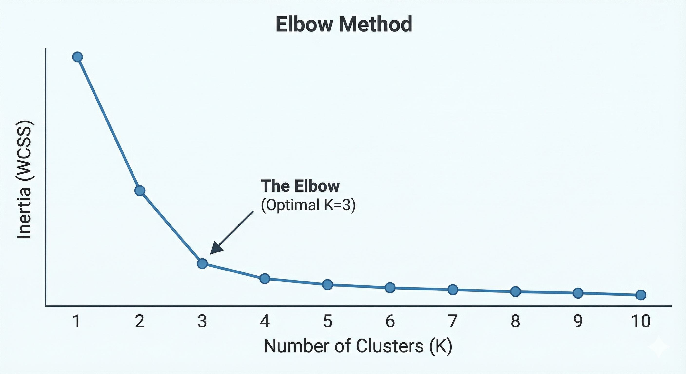
Figure: The Elbow Method visualized — look for the point of diminishing returns.

By looking at the plot, we see the “bend” or elbow happens at K=3. This confirms that our data naturally falls into three distinct groups.

Step 3: Initialization & Training (Running K-Means)

Now that we have identified the “Optimal K” using the Elbow Method, it’s time to let the AI do its work.

We will initialize the K-Means algorithm with n_clusters=3. In this step, the algorithm will:

1. Place 3 random “centroids” (center points) in our data.
2. Assign every customer to the nearest centroid.
3. Calculate the new center of those assigned points.
4. Move the centroid to that new center and repeat until the groups are stable.

Notice that we still only use .fit(X). There are no labels provided; the model is discovering the boundaries itself.

# --- STEP 3: Initialize and Fit K-Means ---
# We use K=3 as determined by the Elbow Method
kmeans = KMeans(n_clusters=3, random_state=42, n_init=10)

# The model learns the clusters from the data features (X)
# 'y_kmeans' will contain the cluster ID (0, 1, or 2) for each customer
y_kmeans = kmeans.fit_predict(X)

print("Cluster IDs assigned to the first 5 customers:", y_kmeans[:5])

Step 4: Visualization (Seeing the Hidden Order)

Data science is often about storytelling. While the computer “sees” these clusters in the form of numbers (Cluster IDs), we need to see them visually to confirm they make sense.

We will plot the data points again, but this time we will color-code them according to the Cluster ID assigned by the K-Means algorithm. We will also plot the Centroids—the mathematical centers of each group.

# --- STEP 4: Visualize the Clusters ---
plt.figure(figsize=(10, 7))

# Plotting the three clusters (correct indexing for x and y)
plt.scatter(X[y_kmeans == 0, 0], X[y_kmeans == 0, 1], s=50, c='red', label='Cluster 1 (Budget)')
plt.scatter(X[y_kmeans == 1, 0], X[y_kmeans == 1, 1], s=50, c='blue', label='Cluster 2 (Premium)')
plt.scatter(X[y_kmeans == 2, 0], X[y_kmeans == 2, 1], s=50, c='green', label='Cluster 3 (Standard)')

# Plotting the Centroids (the centers of the clusters)
plt.scatter(kmeans.cluster_centers_[:, 0], kmeans.cluster_centers_[:, 1],
            s=200, c='yellow', marker='X', edgecolors='black', label='Centroids')

plt.title("Customer Segments Identified by Unsupervised Learning")
plt.xlabel("Annual Income (k$)")
plt.ylabel("Spending Score (1-100)")
plt.legend()
plt.grid(True, linestyle='--', alpha=0.6)
plt.show()

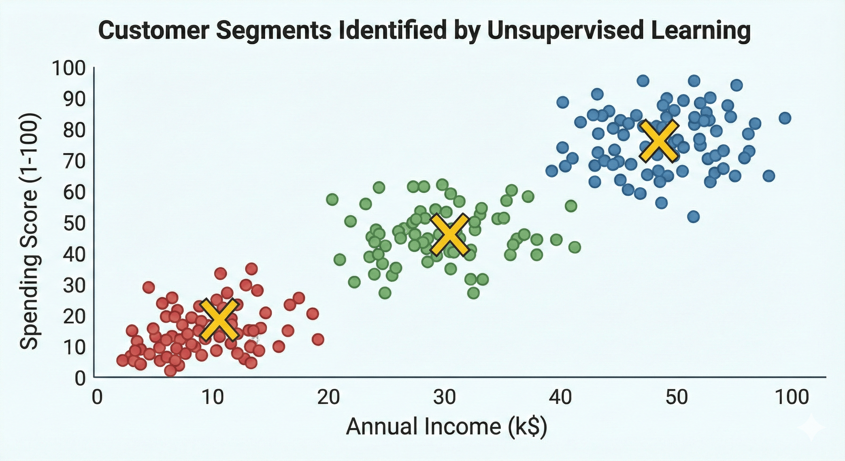
Figure: Final cluster visualization — centroids and colored segments.

Step 5: Interpretation (What did the AI find?)

In Supervised Learning, we knew the labels beforehand. In Unsupervised Learning, the AI gives us the clusters, but we have to give them a name.

Looking at our final visualization, we can now make business decisions based on the three “shopper personas” the model discovered:

1. Cluster 1 (Red): Low income and Low spending score. These are our “Budget Seekers.” They are price-sensitive and likely only come in for essentials or sales.
2. Cluster 2 (Blue): High income and High spending score. These are our “Premium Shoppers.” These are high-value customers who respond well to luxury items and loyalty programs.
3. Cluster 3 (Green): Mid-range income and Mid-range spending. These are our “Standard Staples.” They are consistent, reliable shoppers who likely comprise the bulk of our daily foot traffic.

Without any manual tagging, the AI has successfully segmented our database, allowing us to send targeted marketing emails to each group.

Conclusion: From Chaos to Insight

Unsupervised Learning is perhaps the most “human-like” form of machine intelligence. It represents our ability to walk into a room full of strangers and naturally identify the “groups”—the people laughing in the corner, the people hovering near the buffet, and the people deep in technical debate.

While Supervised Learning is great for predicting the future based on the past, Unsupervised Learning is essential for discovering the present.

It is the tool we use when we don’t even know what questions to ask yet. It’s how we find anomalies in network traffic to stop hackers, how we discover new sub-species in biology, and how we map the stars in distant galaxies.