In the sprawling landscape of Artificial Intelligence and Machine Learning, it’s easy to get lost in buzzwords. You hear about Generative AI, Reinforcement Learning, and Neural Networks.
But before you can run, you must walk. And in the world of ML, “walking” is Supervised Learning.
Supervised Learning is the workhorse of the AI industry. It is the most mature, most widely used, and commercially successful type of machine learning today. From the spam filter in your Gmail to the Face ID on your iPhone, and the algorithm that detected fraud on your credit card transaction yesterday—it’s almost certainly Supervised Learning under the hood.
If you want to understand how machines actually “learn,” you must start here.
This guide is designed to take you from zero knowledge to building your own supervised model. We will start with a simple, non-technical explanation, move into the technical mechanics, and finally, get our hands dirty with Python code.
Part 1: The Non-Technical Explanation (The Analogy)
How do humans learn?
Sometimes, we learn by exploring. A toddler touches a hot stove, feels pain, and learns not to do it again. That is Reinforcement Learning (learning through consequence).
Other times, we learn by finding patterns on our own. You might look at a thousand abstract paintings and realize they naturally fall into three distinct styles, even if you don’t know the names of those styles. That is Unsupervised Learning (finding hidden structures without guidance).
Supervised Learning is different. It is learning with a teacher, a guide, or an answer key.
The “Flashcard” Analogy
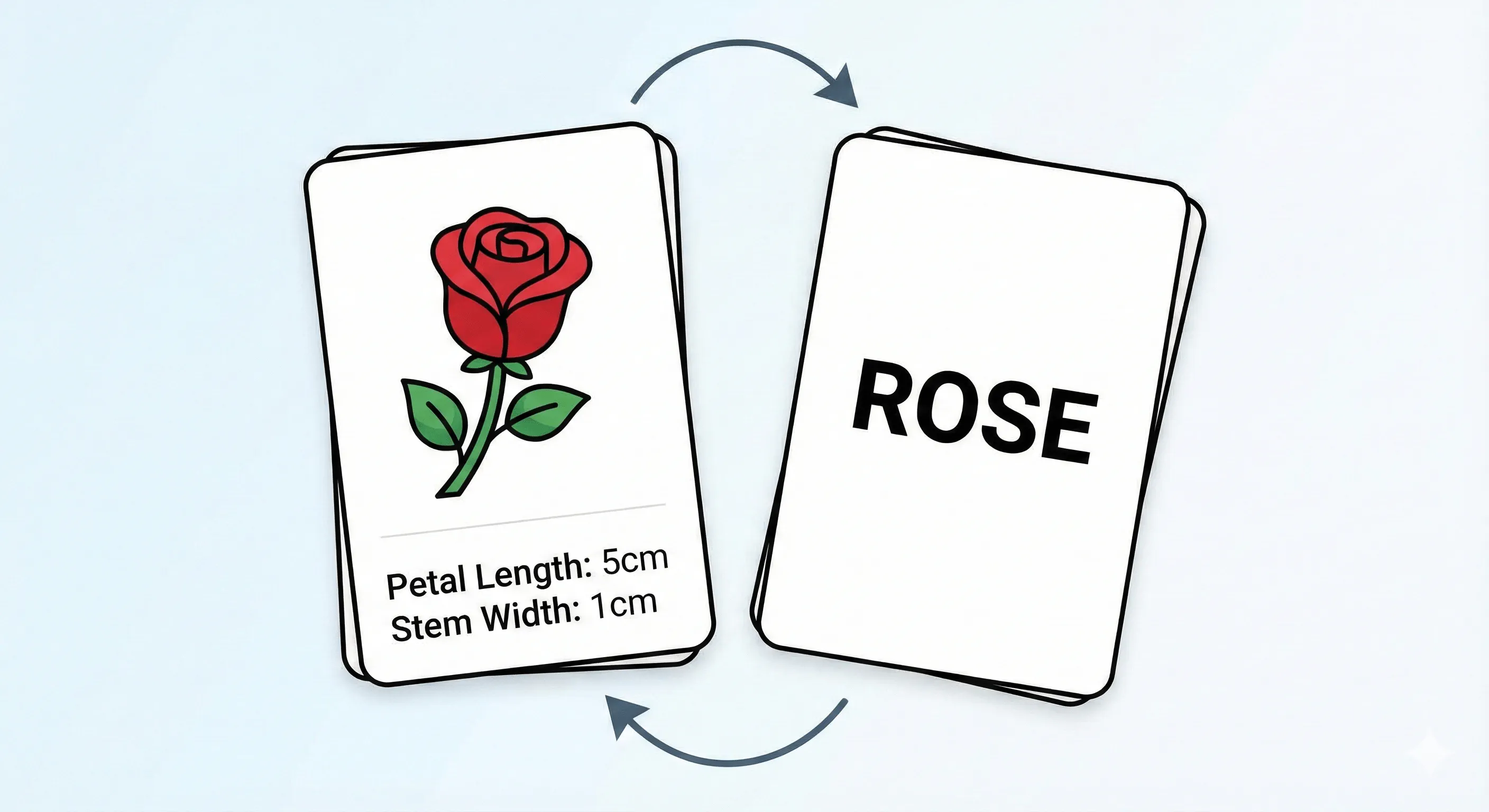
Imagine you are studying for a difficult exam on identifying different species of flowers. You have a stack of 1,000 flashcards.
On the front of each card is a picture of a flower and some data points: petal length, color, and stem width. On the back of the card is the correct answer: “Rose,” “Sunflower,” or “Tulip.”
How do you study?
- You look at the picture and data on the front (the Input).
- You make a guess about what flower it is.
- You flip the card over to see the correct answer (the Label).
- If you were wrong, your brain adjusts. You tell yourself, “Okay, the red ones with short stems aren’t always roses; I need to look closer at the petal shape next time.”
You repeat this process hundreds of times. Eventually, your brain gets very good at mapping the patterns on the front of the card to the answer on the back. You can then pick up a new flower you’ve never seen before and correctly identify it.
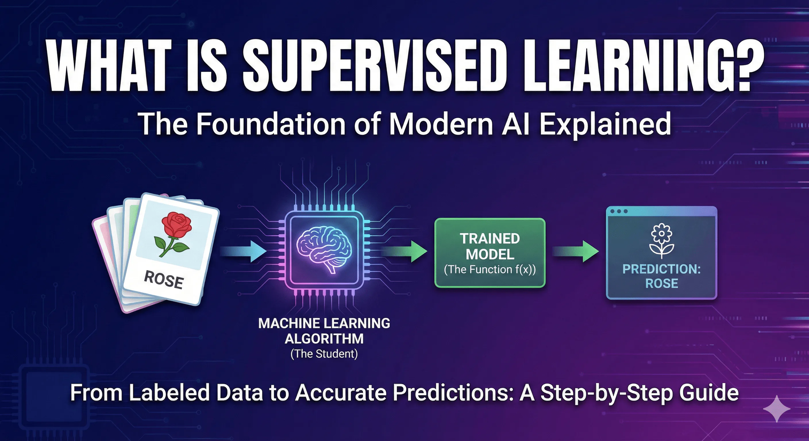
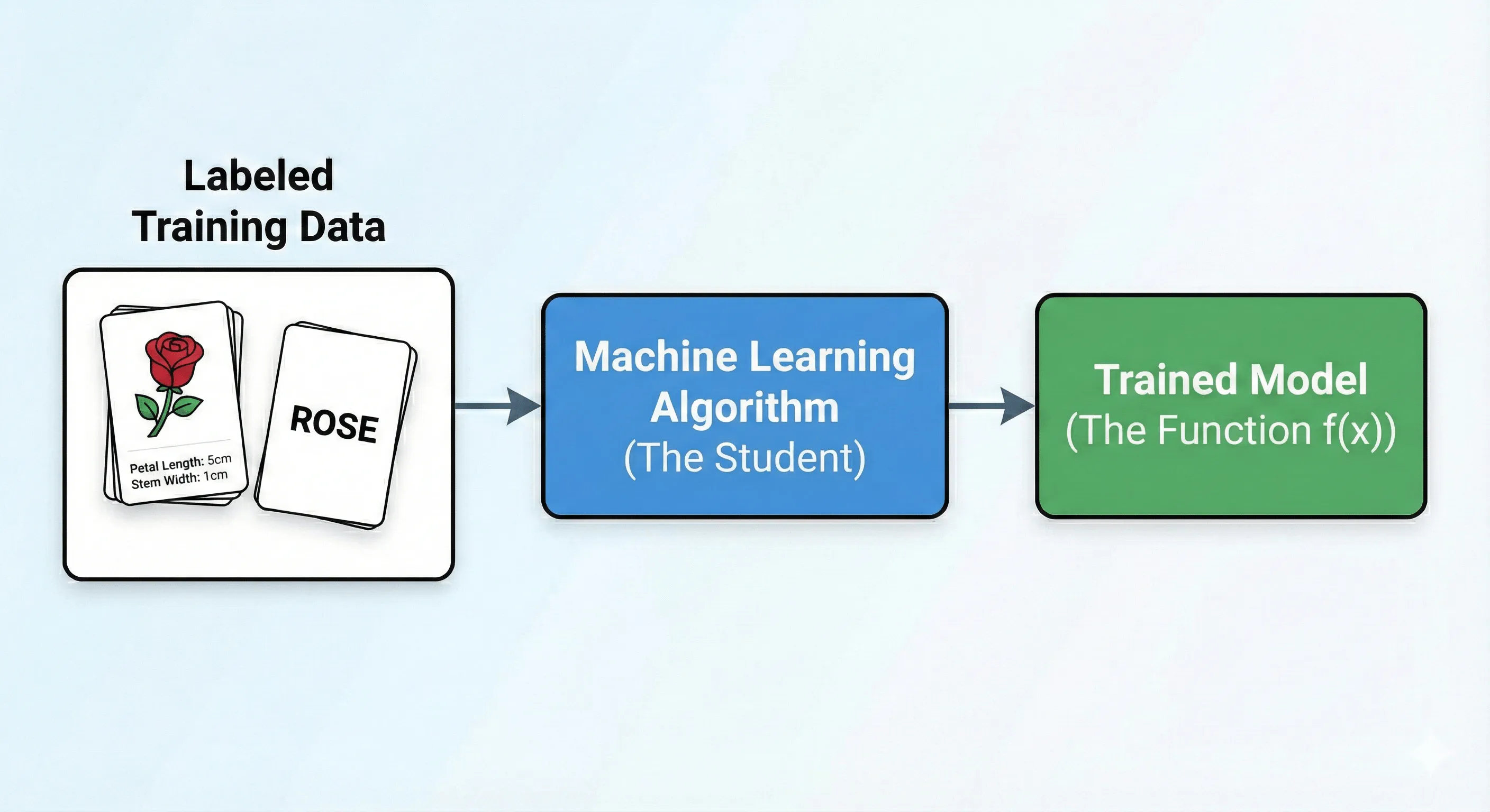
In machine learning, the computer is the student, and the “labeled dataset” is the stack of flashcards.
Supervised learning is simply the process of showing a computer massive amounts of data where we already know the correct answer, and asking it to figure out the relationship between the two.
Part 2: The Technical Deep Dive
Now, let’s tighten up our language. In data science, we don’t talk about “flashcards” and “answers on the back.” We use precise terminology.
Supervised Learning is defined by the use of Labeled Data.
Data is considered “labeled” when it consists of paired examples: the input data that the model will analyze, and the desired output value that the model should predict.
The Anatomy of Labeled Data
To train a supervised model, your data must be structured into two distinct parts:
1. Features (Inputs / Independent Variables / $X$) These are the characteristics of the data point that you want the model to analyze.
- In our flower example: Petal length, color, stem width.
- In predicting house prices: Square footage, number of bedrooms, zip code.
- In email filtering: The words in the subject line, the sender’s address.
2. Labels (Targets / Outputs / Dependent Variables / $y$) This is the “correct answer” you want the model to learn to predict.
- In our flower example: “Rose.”
- In predicting house prices: $450,000.
- In email filtering: “Spam” or “Not Spam.”
The Goal: Finding the “Mapping Function”
Mathematically, the goal of supervised learning is deceptively simple.
We have input variables ($X$) and output variables ($y$). We are trying to find a mathematical function ($f$) that maps the input to the output so accurately that when we have new input data ($X_{new}$) where we don’t know the answer, we can predict it ($y_{pred}$).
$$y = f(X)$$
The “learning” part is the process of an algorithm autonomously adjusting its internal parameters to find the best possible version of that function $f$. It does this by making predictions on training data, comparing its prediction to the actual label, calculating how wrong it was (the “loss” or “error”), and adjusting itself to be slightly less wrong next time.
Two Main Flavors: Regression vs. Classification
Not all supervised learning tasks are the same. They generally fall into two major categories based on the type of answer (Label) you are trying to predict.
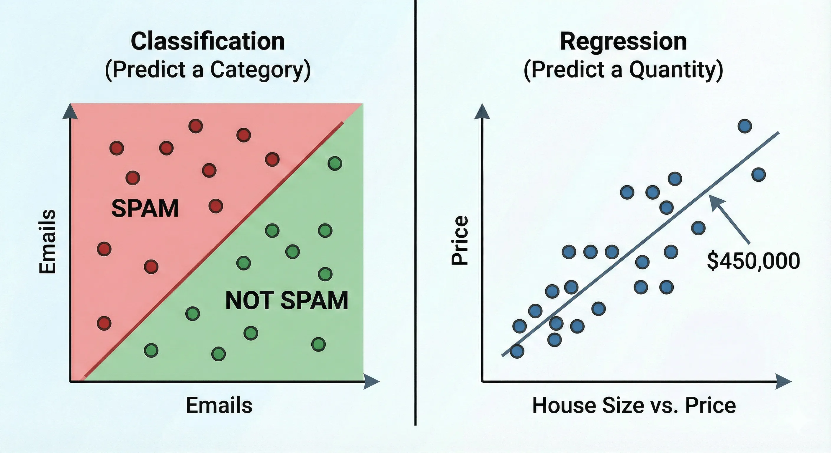
1. Classification (Predicting a Category) The output variable is a category or a class. The answers are discrete patches.
- Is this email Spam or Not Spam? (Binary Classification)
- Is this image a Cat, a Dog, or a Horse? (Multi-class Classification)
- Will this customer Churn (leave) or Stay?
2. Regression (Predicting a Quantity) The output variable is a continuous numerical value. The answers are on a sliding scale.
- What will be the price of this house next year?
- What will the temperature be tomorrow?
- How many units of this product will we sell next month?
Part 3: The Coding Tutorial — Building a Supervised Model
Enough theory. The best way to understand this is to do it.
We are going to build a simple Binary Classification model.
The Scenario: Imagine we are an online video platform. We want to predict if a user will “Like” a movie based on just two features:
- The User’s Age.
- The Movie’s Runtime (in minutes).
Note: In the real world, we would use thousands of features, but we will keep it simple to see the mechanics.
We will use Python and the industry-standard library scikit-learn (sklearn).
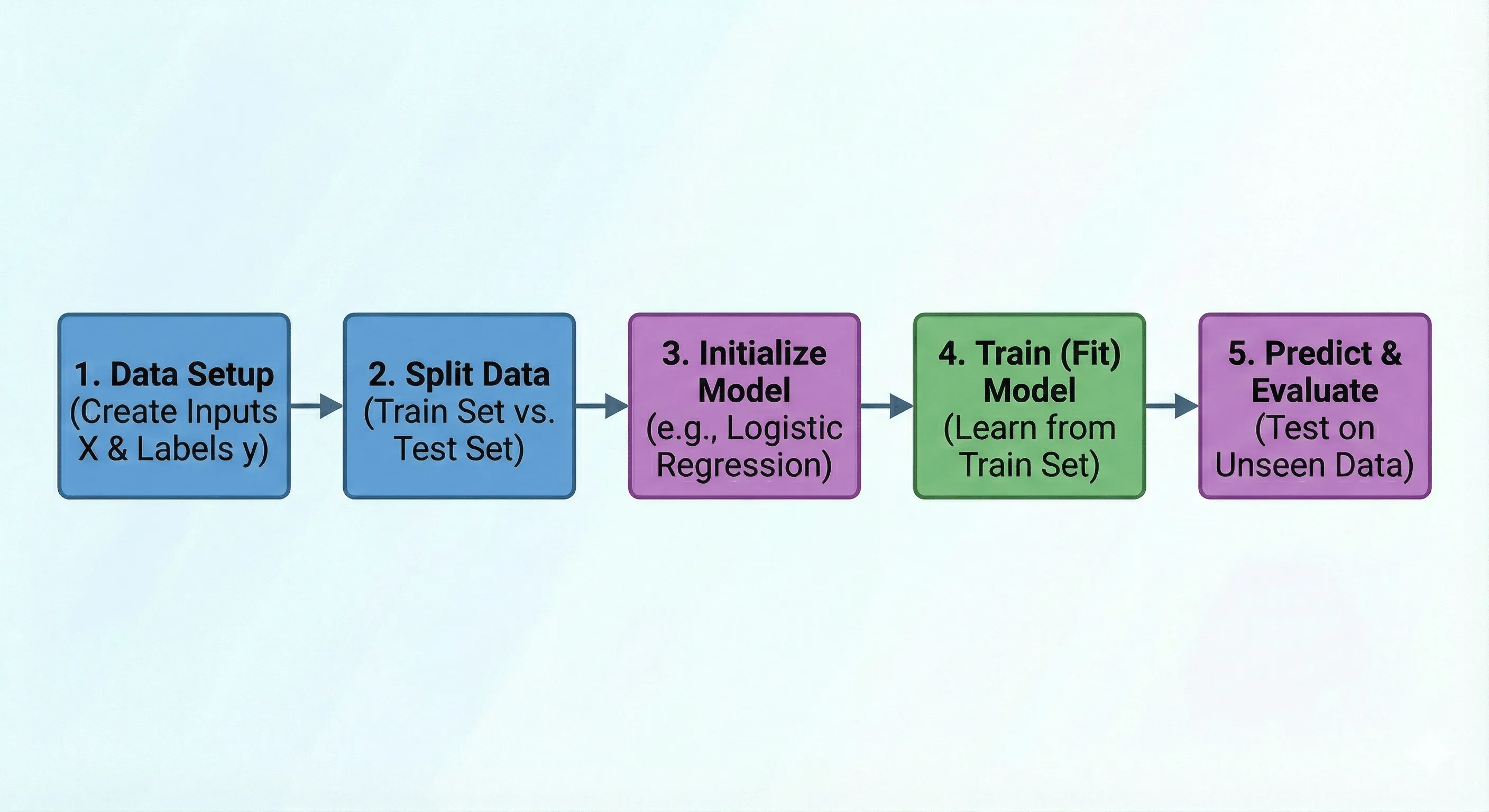
We will break this process down into 5 distinct steps:
- Data Setup: Creating our synthetic labeled data.
- Splitting: Separating data for training versus testing.
- Initialization: Choosing our model.
- Training (Fitting): The learning process.
- Prediction & Evaluation: Seeing how well it worked.
Step 1: Data Setup
First, we need to import necessary libraries and create some synthetic data that represents our “flashcards.” We will create inputs ($X$) representing Age and Runtime, and corresponding labels ($y$) representing 0 for “Did Not Like” and 1 for “Liked”.
import numpy as np
from sklearn.model_selection import train_test_split
from sklearn.linear_model import LogisticRegression
from sklearn.metrics import accuracy_score

# --- STEP 1: Create Synthetic Data ---
# We are creating a small dataset of 20 samples.
# X = Features (Age, Runtime in minutes)
# y = Labels (0 = Did Not Like, 1 = Liked)

# Feature 1: Age (ranging from ~18 to ~65)
# Feature 2: Movie Runtime (ranging from ~90 to ~180 minutes)
X_data = np.array([
    [22, 95],  [25, 110], [45, 120], [50, 105], [60, 160],
    [19, 90],  [30, 100], [35, 130], [55, 115], [62, 170],
    [28, 140], [40, 150], [48, 125], [52, 135], [21, 100],
    [24, 110], [42, 145], [58, 155], [32, 120], [38, 130]
])

# Labels (Target): 0 or 1
# Let's assume a pattern where older users prefer longer movies.
# This label data is manually handcrafted to create a learnable pattern.
y_data = np.array([
    0, 0, 1, 1, 1,
    0, 0, 1, 1, 1,
    0, 1, 1, 1, 0,
    0, 1, 1, 0, 1
])

print(f"Total dataset size: {len(X_data)} samples.")
# Output: Total dataset size: 20 samples.
# --- STEP 2: Split into Train and Test Sets ---
# We split the data: 80% for training, 20% for testing.
# random_state ensures we get the same split every time we run the code.
X_train, X_test, y_train, y_test = train_test_split(
    X_data, y_data, test_size=0.2, random_state=42
)

print(f"Training data size: {len(X_train)} samples.")
print(f"Testing data size: {len(X_test)} samples.")
# Output: Training data size: 16 samples.
# Output: Testing data size: 4 samples.

#### Step 3: Model Initialization

Now we need to choose our student. Which machine learning algorithm will we use to solve this classification problem?

There are many algorithms to choose from—Decision Trees, Support Vector Machines, Naive Bayes, Random Forests.
For this simple binary classification task, we will use **Logistic Regression**.
Despite its name containing "regression," it's a powerful and widely used algorithm for classification.

We initialize it by creating an "instance" of the model. At this point, it's like a student on their first day of class:
it knows *how* to learn, but it hasn't learned anything yet.

```python
# --- STEP 3: Initialize the Model ---
# We will use Logistic Regression, a common algorithm for binary classification.
# At this point, the model is "untrained" with default parameters.
model = LogisticRegression()

# --- STEP 4: Train (Fit) the Model ---
# The .fit() method is where the learning happens.
# The model finds the relationship between the features (X_train)
# and the labels (y_train).
print("Training model...")
model.fit(X_train, y_train)
print("Model trained successfully!")
# Output:
# Training model...
# Model trained successfully!

# --- STEP 5: Predict & Evaluate ---
# Predict on the test set and compute accuracy
y_pred = model.predict(X_test)
acc = accuracy_score(y_test, y_pred)
print(f"Test Accuracy: {acc:.2f}")

# Example: single-sample prediction
sample = np.array([[30, 125]])  # Age=30, Runtime=125
pred = model.predict(sample)
print(f"Sample prediction (Age 30, Runtime 125): {'Liked' if pred[0]==1 else 'Did not like'}")
