We have covered Supervised Learning, where a “teacher” provides the correct answers (labels). We have covered Unsupervised Learning, where an “explorer” finds hidden patterns in static piles of data.
But what if there is no teacher? And what if the data isn’t just sitting in a database, but is being generated live by the world around you?
What if you want to teach a robot to walk, a computer to play chess, or an AI to optimize a supply chain?
In these scenarios, the “correct answer” isn’t immediately obvious. A move in chess might seem good now but lead to a loss twenty turns later. A robot might take a step that looks stable but causes it to fall over two seconds later.
This is the domain of Reinforcement Learning (RL). It is the closest analogy we have to how biological beings learn complex skills. It is learning through interaction, consequence, and the relentless pursuit of a reward.
Part 1: The Non-Technical Analogy (Training a Puppy)
Forget computers for a second. Imagine you have just adopted a new puppy. You want to teach it to “sit.”
How do you do it?
You don’t have a USB cable to plug into its brain to upload the “sit” command. You cannot show it 10,000 flashcards of other dogs sitting.
Instead, you use a system of rewards and penalties (mostly rewards, hopefully).
- The Situation: You are in the living room. The puppy is standing looking at you.
- The Action: You say “Sit.” The puppy looks confused. It wanders around. It sniffs the carpet. It jumps on your leg.
- The Feedback: Nothing happens.
- The Accidental Success: Eventually, randomly, its butt hits the floor.
- The Reward: Immediately, you say “Good boy!” and give it a treat.
The puppy’s brain makes a connection: When I am in the living room (State) and I hear the sound “Sit”, if I lower my rear end (Action), I get a delicious treat (Reward).
You repeat this dozens of times. Eventually, the puppy learns the Policy: When “Sit” command hears, put butt on floor to maximize future treats.
This is Reinforcement Learning.
The puppy is the Agent. The living room is the Environment. The treat is the Reward Signal. The puppy learns through trial and error which actions yield the best long-term rewards.
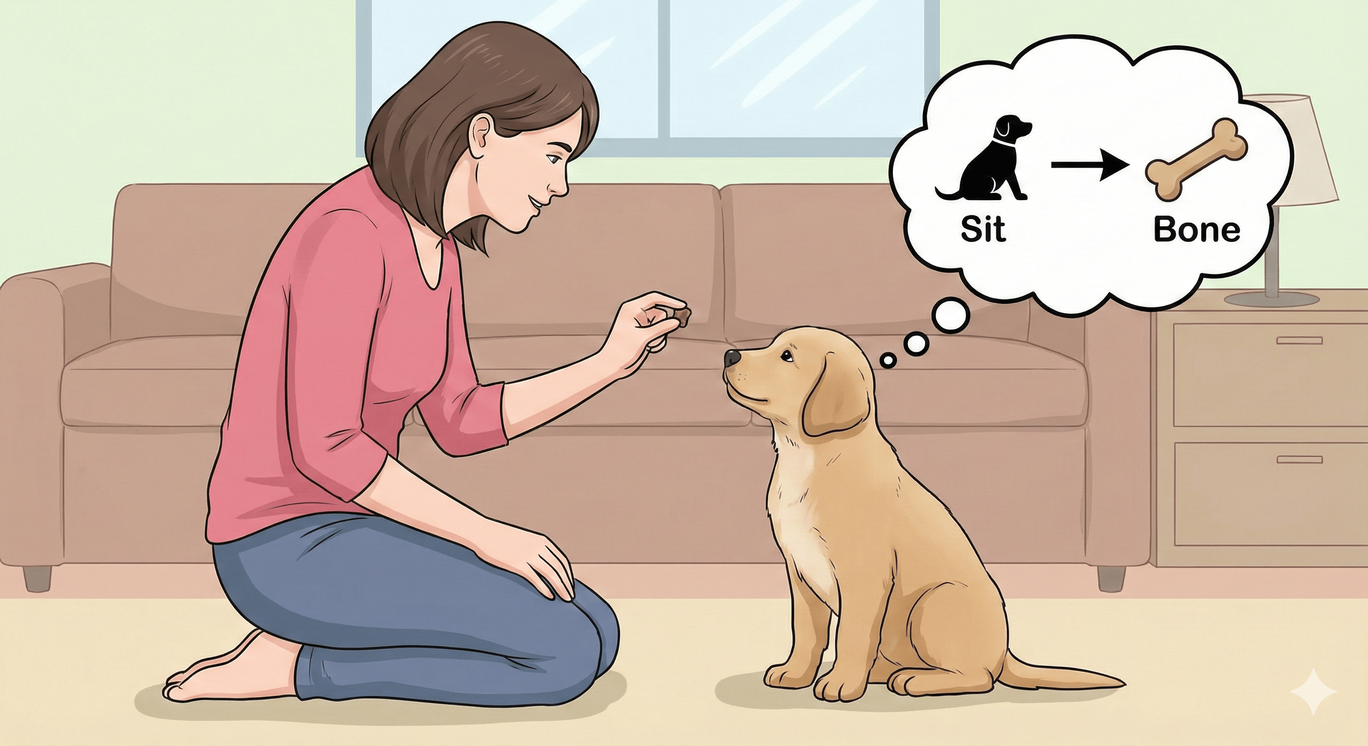 The Analogy: Training a Puppy — learning by reward and consequence.
Part 2: The Technical Deep Dive (The RL Loop)
In technical terms, Reinforcement Learning is a computational approach to learning whereby an agent learns to make decisions by performing actions in an environment and receiving feedback in the form of rewards or penalties.
Unlike supervised learning, the feedback is delayed. The agent doesn’t know if an action was truly “correct” until much later.
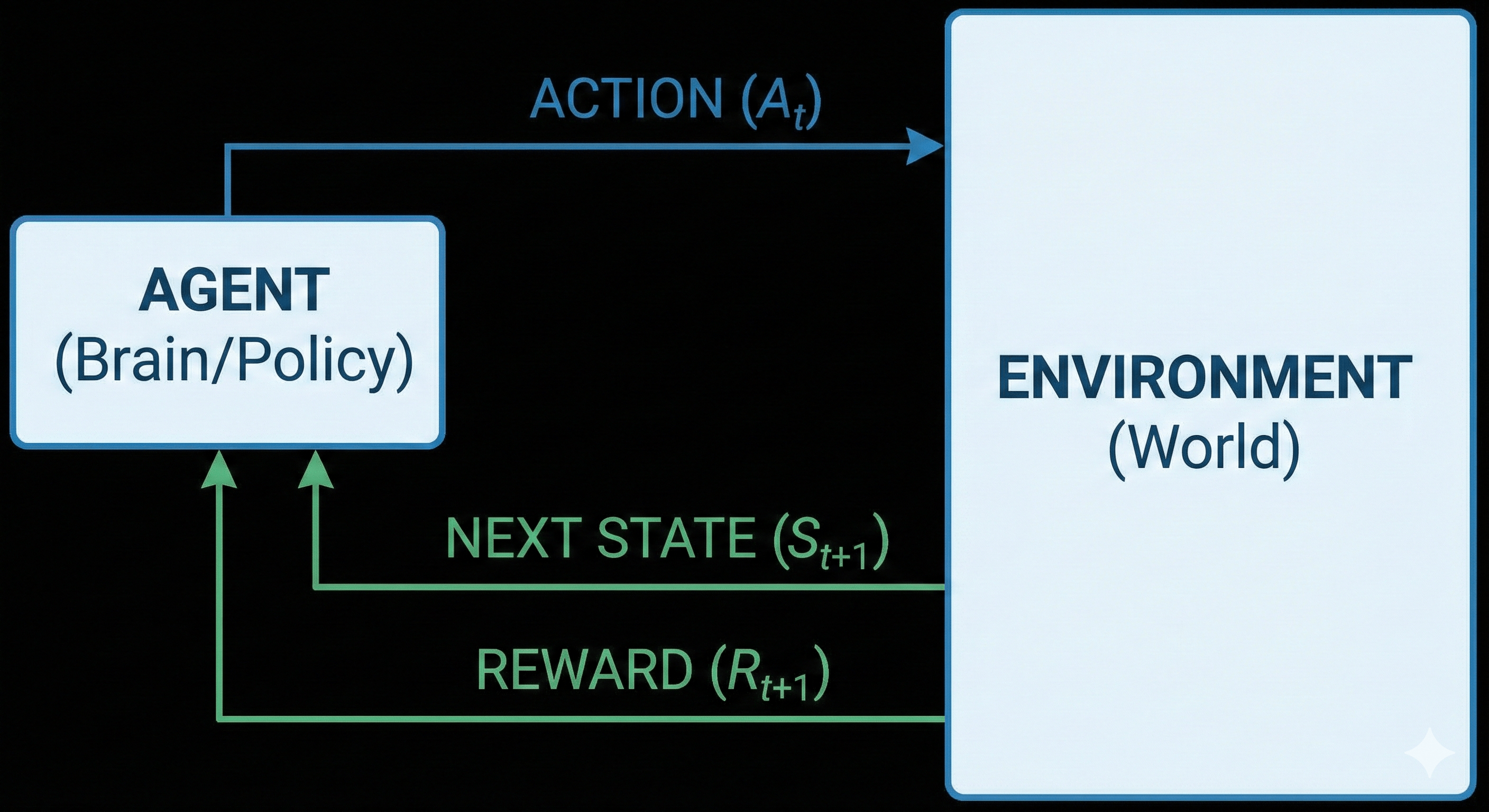 The Technical Concept: The RL Loop — agent, action, state, reward, repeat.
The Vocabulary of RL
To understand RL, you must understand the fundamental feedback loop that happens at every time step:
- Agent: The learner and decision-maker (e.g., the chess-playing AI, the robot).
- Environment: Everything the agent interacts with (e.g., the chess board and rules, the physical laws of gravity).
- State ($S_t$): A snapshot of the current situation at time $t$. (Where am I now?)
- Action ($A_t$): The move the agent chooses to make. (What do I do next?)
- Reward ($R_{t+1}$): A numerical scalar signal received after taking an action. It tells the agent how good that immediate step was. (+1 for winning, -1 for losing, 0 for nothing happened).
The Goal: The Policy and Cumulative Reward
The agent’s goal isn’t just to get a reward right now. It’s to maximize the total cumulative reward over time. Sometimes you have to sacrifice an immediate reward (like sacrificing a pawn in chess) to gain a massive reward later (winning the game).
The solution to an RL problem is finding the optimal Policy ($\pi$).
A policy is the agent’s brain. It is a mapping function from States to Actions. It tells the agent: “If you are in State X, you should take Action Y to have the best chance of maximizing future rewards.”
Part 3: The Coding Tutorial — Q-Learning on a Frozen Lake
RL gets very complicated, very fast, often involving deep neural networks (Deep Q-Networks or PPO).
However, the fundamentals can be learned with a simpler, table-based method called Q-Learning. We don’t need a neural network if the environment is small enough.
The Scenario: FrozenLake-v1
We will use the standard Gymnasium library (formerly OpenAI Gym). We will tackle the “FrozenLake” environment.
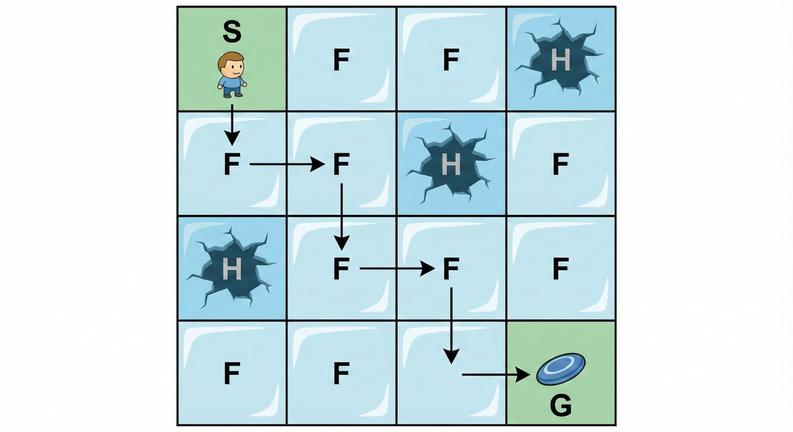
Imagine a 4x4 grid.
- S: Start point (safe)
- F: Frozen surface (safe to walk on)
- H: Hole (you fall in and die)
- G: Goal (the frisbee, where the reward is)
The agent wants to get from S to G without falling into an H. The ice is slippery, so sometimes if you try to move right, you might slide down instead.
The Goal: Teach an agent to navigate this slippery grid purely by falling into holes until it figures it out.
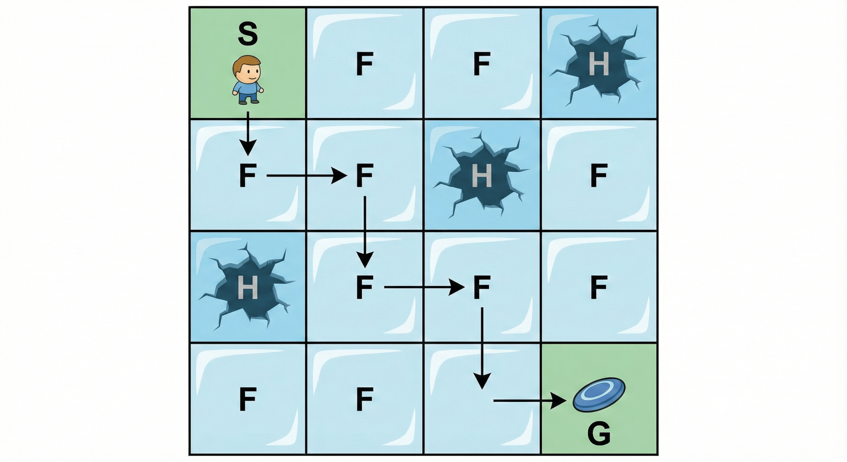 The FrozenLake 4x4 grid: S = Start, F = Frozen, H = Hole, G = Goal.
Step 1: Setup the Environment
First, install the necessary library:
pip install "gymnasium[toy-text]"
Now, let’s initialize the environment and see what it looks like.
Beginning with the code for setting up the environment.
import numpy as np
import gymnasium as gym
import random

# --- STEP 1: Setup the Environment ---
# We use the 'FrozenLake-v1' environment.
# map_name="4x4": A small 16-tile grid.
# is_slippery=False: To keep it simple first. If True, the agent slips randomly.
# render_mode=None: We don't want to see pop-up windows during fast training.

env = gym.make("FrozenLake-v1", map_name="4x4", is_slippery=False, render_mode=None)

# Let's inspect what we are working with
state_space = env.observation_space.n
action_space = env.action_space.n

print(f"Number of States: {state_space} (The 16 tiles on the grid)")
print(f"Number of Actions: {action_space} (Left, Down, Right, Up)")
Step 2: The Q-Table (The “Cheat Sheet”)
The heart of Q-Learning is the Q-Table.
Imagine a spreadsheet.
- The Rows represent every possible State (0 to 15, representing the 16 tiles).
- The Columns represent every possible Action (0 to 3: Left, Down, Right, Up).
- The Cells contain the “Q-Value” (Quality Value). This number represents: “If I am in this state and I take this action, how much future reward can I expect?”
At the beginning, the agent knows nothing. It has never seen the ice. So, we initialize the entire table with Zeros.
We also need to define our Hyperparameters—the settings that control how the brain learns.
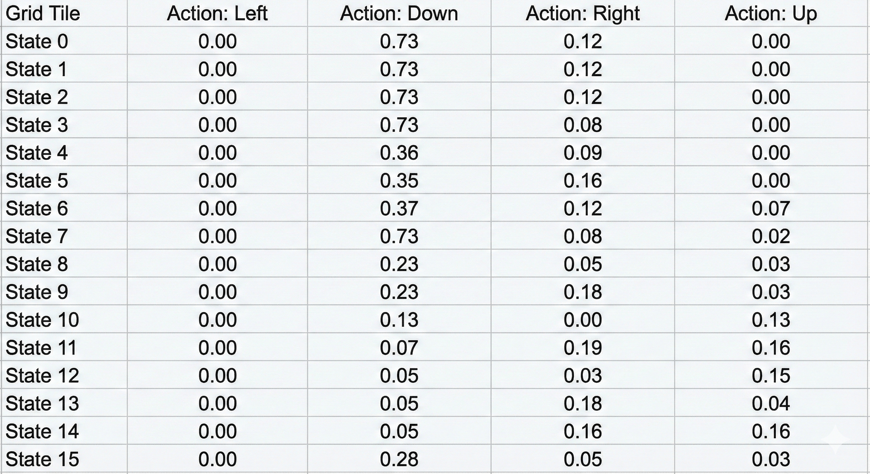 The Q-Table: rows = states, columns = actions, cells = expected future reward (Q-values).
# --- STEP 2: Initialize Q-Table and Hyperparameters ---

# Initialize the Q-Table with zeros
# Dimensions: [16 rows x 4 columns]
q_table = np.zeros((state_space, action_space))

# Hyperparameters
total_episodes = 2000        # How many times we play the game to learn
learning_rate = 0.8          # Alpha: How much we accept new information
discount_factor = 0.95       # Gamma: How much we care about long-term vs short-term reward
epsilon = 1.0                # Exploration Rate: 1.0 = 100% Random exploration at start
max_epsilon = 1.0            # Max exploration probability
min_epsilon = 0.01           # Min exploration probability (at the end)
decay_rate = 0.005           # How fast we stop exploring and start exploiting

print("Q-Table Initialized. Shape:", q_table.shape)
# Output: Q-Table Initialized. Shape: (16, 4)
Step 3: The Training Loop (The “Game of Life”)
This is where the agent actually plays the game 2,000 times.
In every step of every game, the agent faces a fundamental dilemma known as Exploration vs. Exploitation.
- Exploration: Should I try a random move to see what happens? (Maybe I find a shortcut?)
- Exploitation: Should I stick to what I already know works? (I know going Down is safe, so I’ll do that.)
We handle this with epsilon. At the start, epsilon is 1.0 (100%), so the agent moves completely randomly. Over time, we “decay” epsilon, so the agent stops exploring and starts relying on its learned experience (the Q-Table).
Here is the implementation of the Q-Learning algorithm:
# --- STEP 3: The Training Loop ---
rewards = []

for episode in range(total_episodes):
    state, info = env.reset()
    total_rewards = 0
    done = False

    while not done:
        # A. CHOOSE ACTION (Explore vs Exploit)
        # Generate a random number. If it's smaller than epsilon, we explore (random action)
        if random.uniform(0, 1) < epsilon:
            action = env.action_space.sample()
        else:
            # Otherwise, we exploit (choose the best known action for this state)
            action = np.argmax(q_table[state, :])

        # B. TAKE ACTION
        # The environment returns:
        # new_state: Where we landed
        # reward: Did we get a treat? (+1 for Goal, 0 otherwise)
        # done: Did we fall in a hole or reach the goal?
        new_state, reward, terminated, truncated, info = env.step(action)
        done = terminated or truncated

        # C. UPDATE Q-TABLE (The Learning Part)
        # This is the Bellman Equation implementation.
        # It updates the cell for the current state/action with a mix of:
        # 1. The old value (memory)
        # 2. The immediate reward just received
        # 3. The best possible future reward from the NEW state (looking ahead)

        q_table[state, action] = q_table[state, action] + learning_rate * (
            reward + discount_factor * np.max(q_table[new_state, :]) - q_table[state, action]
        )

        # D. MOVE TO NEXT STATE
        state = new_state
        total_rewards += reward

    # Reduce epsilon (Decay)
    # As we play more, we explore less and trust our table more
    epsilon = min_epsilon + (max_epsilon - min_epsilon) * np.exp(-decay_rate * episode)
    rewards.append(total_rewards)

print("Training finished!")
print(f"Q-Table updated. Values at Start State (0):\n{q_table[0]}")
# Output will show non-zero numbers, indicating the agent learned something about the start.
The mathematical formula inside comment Section C is the magic. It effectively says: “The value of this step is equal to the immediate reward I got plus the maximum potential value of the future situation I landed in.”
This allows rewards to “propagate” backward from the Goal to the Start. Even though the step Start -> Down gives 0 immediate reward, the Q-table learns it is valuable because it eventually leads to the Goal.
Step 4: Evaluation (Watch it Play)
Now that the training is done, our Q-Table should be a perfect “cheat sheet.” To test it, we turn off the randomness (Exploration) completely. We tell the agent: “Don’t try anything new. Just look at the table and do exactly what it says is best.”
We will run 5 test games to see if the agent can survive the frozen lake every time.
# --- STEP 4: Evaluation ---
# Run the game 5 times using the trained Q-Table
env = gym.make("FrozenLake-v1", map_name="4x4", is_slippery=False, render_mode="human")

for episode in range(5):
    state, info = env.reset()
    done = False
    print(f"--- EPISODE {episode+1} ---")

    for step in range(20): # Max 20 steps to prevent infinite loops
        # Choose the action with the highest value in the Q-Table
        # No randomness here!
        action = np.argmax(q_table[state, :])

        # Take the action
        new_state, reward, terminated, truncated, info = env.step(action)
        done = terminated or truncated

        if done:
            env.render()
            if reward == 1:
                print("You reached the Goal! 🏆")
            else:
                print("You fell in a hole! ☠️")
            break

        state = new_state

env.close()
When you run this code locally, you will see a window pop up showing the little elf navigating the grid perfectly, avoiding holes and grabbing the frisbee every single time. It has “solved” the environment.
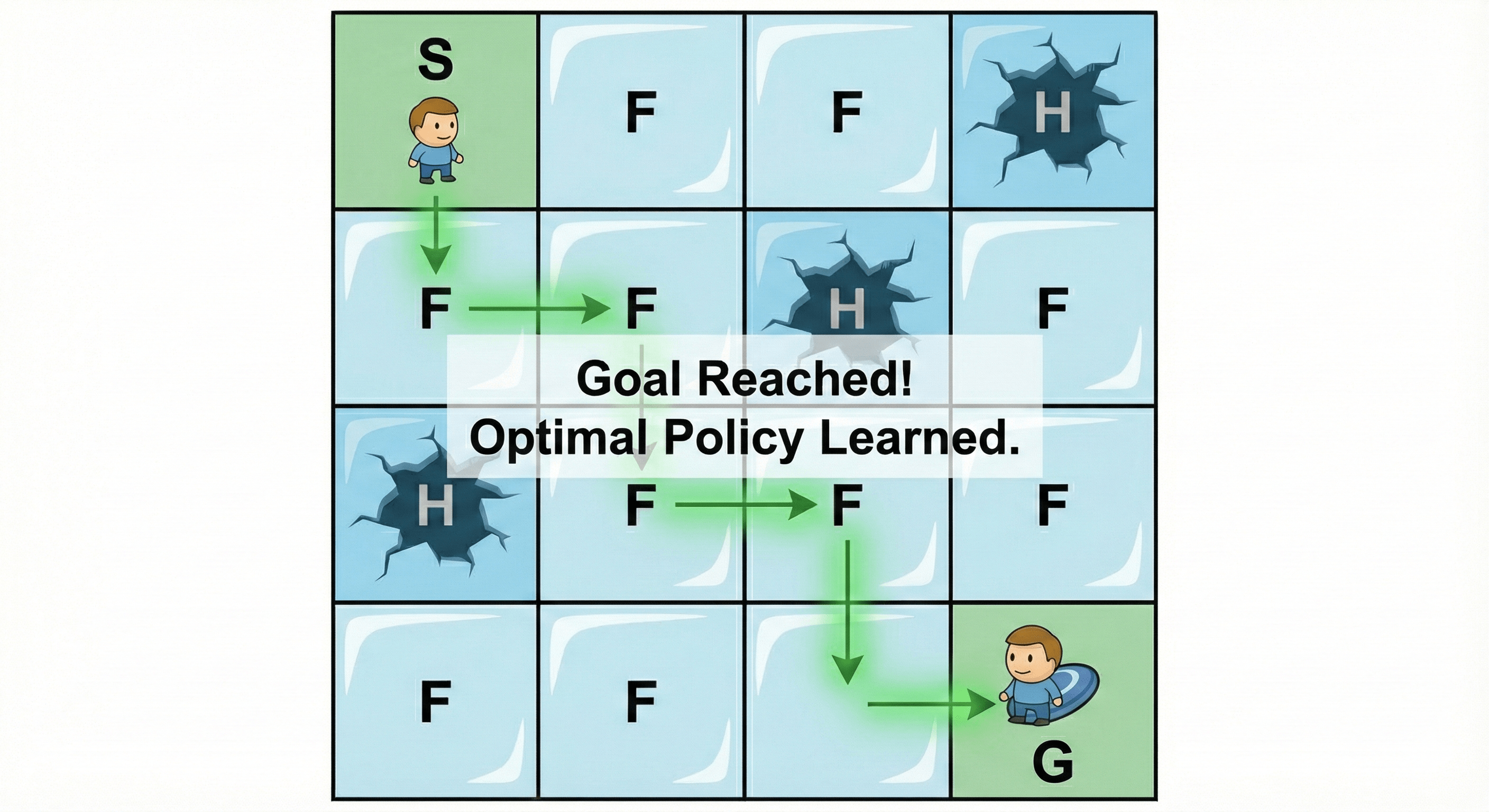 The Successful Outcome — agent follows the learned optimal path from Start to Goal.
Step 5: Interpretation (Reading the Brain)
If we print out the final Q-Table, we can actually see what the agent “thinks.”
The table is just a grid of numbers. If row 0 (Start State) looks like this:
[0.59, 0.73, 0.59, 0.55]
It means the agent values action 1 (Down) the highest (). Why? Because moving Down from the start is the safest first step toward the goal in this specific map. The agent doesn’t know why (it doesn’t understand “gravity” or “holes”), it just knows that mathematically, “Down” yields the highest probability of a future reward.
Conclusion: The Holy Trinity of AI
Congratulations! You have now built models for the three pillars of Machine Learning:
- Supervised Learning: The Student. Learning from labeled flashcards (Input Output).
- Unsupervised Learning: The Explorer. Finding hidden patterns in chaos (Clustering).
- Reinforcement Learning: The Gamer. Learning through trial, error, and reward (Action Consequence).
While the FrozenLake is a simple toy example, the mechanics you just wrote—State, Action, Reward, Policy—are the exact same mechanics used by AlphaGo to beat the world champion at Go, and by Tesla’s autopilot to navigate traffic.