
1: The Question Nobody Asks Early Enough
You have built an AI model. You have collected your data, cleaned it, split it into training and test sets, chosen an architecture, tuned your hyperparameters, and hit “Run.” After hours (or days) of training, the terminal spits out a number:
Accuracy: 96.3%
You feel a wave of relief. You think, “96%! That’s an A+. My model is brilliant. Ship it.”
Stop. Right. There.
That single number—Accuracy—might be the most misleading statistic in all of Machine Learning. Before you deploy that model into production, before you stake your company’s reputation (or a patient’s life) on it, you need to ask a far more fundamental question:
What does “good” even mean?
This is not a philosophical tangent. It is the most practical, career-defining question a Data Scientist or ML Engineer will ever face. Because in the real world, the metric you choose to optimize determines the kind of mistakes your model makes. And in many domains, some mistakes are catastrophically worse than others.
A spam filter that accidentally blocks your boss’s email is annoying. A medical AI that tells a cancer patient they are healthy is lethal.
Both models might report “96% accuracy.” But one is a mild inconvenience, and the other is a death sentence.
In this deep dive, we will unpack the full toolkit of AI evaluation—from the classic metrics of classification (Accuracy, Precision, Recall, F1-Score) to the specialized metrics of language models (Perplexity, BLEU), to the emerging frontier of evaluating generative AI. By the end, you will never look at a single accuracy number the same way again.
2: The Analogy — The Smoke Detector and the Surgeon
Before we touch any math, let’s build intuition with two stories.
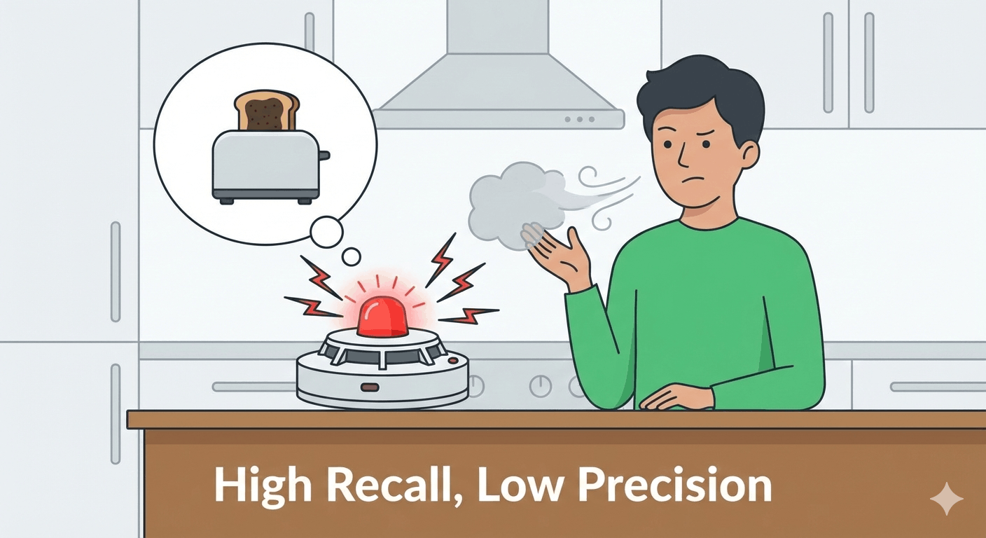
Story A: The Paranoid Smoke Detector
Imagine you install a new, state-of-the-art smoke detector in your kitchen. It is incredibly sensitive. It goes off when there is a real fire. It also goes off when you make toast. And when you boil water. And when you open the oven. And sometimes, just for fun, at 3 AM when nothing is happening.
Is this smoke detector “good”?
Well, it has never missed a real fire. Every single time there has been smoke from an actual dangerous source, it has caught it. In that sense, its detection rate for real fires is 100%. It never lets a fire slip by undetected.
But you hate it. Because 95% of the time, it is screaming about toast. It is so sensitive that it flags everything, and you have started ignoring it entirely. You have ripped the batteries out. Now if a real fire happens, you won’t hear the alarm at all.
The core issue: The detector catches everything, but it also cries wolf constantly. It has high Recall (catches all real fires) but low Precision (most of its alarms are false).
Story B: The Overconfident Surgeon
Now imagine a different scenario. You go to a surgeon for a biopsy. The surgeon looks at your results and says, “You’re fine. No cancer.” You feel relieved.
But here’s the catch: this particular surgeon has a policy. She is extremely conservative. She only diagnoses cancer when she is absolutely, 100% certain. If there is even a 1% chance the tissue is benign, she says “no cancer.”
The result? When she does say “cancer,” she is almost always right. Her positive diagnoses are highly trustworthy. But she misses a lot of actual cancers because she is too cautious. She sends early-stage patients home with a clean bill of health, and they return a year later with Stage 4 tumors.
The core issue: When she speaks, she is almost always correct. But she stays silent too often, missing real cases. She has high Precision (when she says cancer, it’s cancer) but low Recall (she misses many actual cancers).
The Lesson
These two stories illustrate the fundamental trade-off in AI evaluation:
- Precision answers: “When the model says YES, how often is it actually correct?”
- Recall answers: “Of all the actual YES cases in the world, how many did the model find?”
You cannot maximize both simultaneously. Increasing one typically decreases the other. The art of ML engineering is deciding which type of mistake is more acceptable for your specific use case.
| Scenario | Worse Mistake | Optimize For |
|---|---|---|
| Cancer Detection | Missing a real cancer (False Negative) | Recall (Catch them all) |
| Spam Filter | Blocking a real email (False Positive) | Precision (Don’t cry wolf) |
| Self-Driving Car | Not detecting a pedestrian | Recall |
| Legal Document Review | Flagging irrelevant docs as relevant | Precision |
| Fraud Detection | Missing actual fraud | Recall |
This is why “accuracy” alone is meaningless. It tells you nothing about what kind of errors your model is making.
3: The Foundation — The Confusion Matrix
Every classification metric in existence is derived from one beautifully simple table called the Confusion Matrix. If you understand this table, you understand everything.
Let’s set up a concrete scenario. You have built a model that looks at medical images and predicts: “Cancer” or “Not Cancer.”
You run it on 1,000 test images where you already know the true answer.
The Confusion Matrix organizes the results into four buckets:
| Model Says: Cancer | Model Says: Not Cancer | |
|---|---|---|
| Reality: Cancer | True Positive (TP) = 80 | False Negative (FN) = 20 |
| Reality: Not Cancer | False Positive (FP) = 30 | True Negative (TN) = 870 |
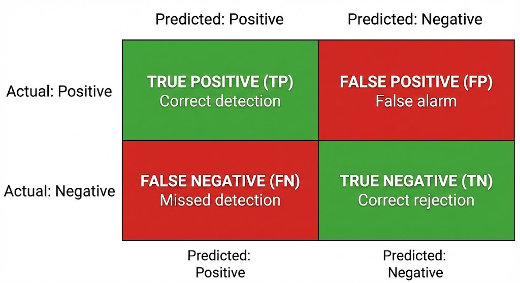
Let’s decode each cell:
True Positive (TP) = 80
The model said “Cancer,” and the patient really has cancer. Correct. This is a hit.
True Negative (TN) = 870
The model said “Not Cancer,” and the patient is truly healthy. Correct. This is also a hit.
False Positive (FP) = 30
The model said “Cancer,” but the patient is actually healthy. Wrong. This is a false alarm. The patient gets terrified, undergoes unnecessary biopsies, and racks up medical bills—all for nothing. This is the “Paranoid Smoke Detector” error.
False Negative (FN) = 20
The model said “Not Cancer,” but the patient actually has cancer. Wrong. This is the silent killer. The patient walks out of the hospital thinking they are healthy, while the tumor continues to grow undetected. This is the “Overconfident Surgeon” error.
Notice something critical: not all errors are equal. In cancer detection, a False Negative (missed cancer) is infinitely worse than a False Positive (false alarm). In a spam filter, it’s the opposite—a False Positive (blocking a real email from your boss) is worse than a False Negative (letting a spam email slip through).
This asymmetry is the entire reason why “accuracy” is insufficient.
4: The Classic Metrics — Dissected
Now that we have the Confusion Matrix, let’s derive every major metric from it. We will use the numbers from the cancer example above.
4.1: Accuracy — The Popular Lie
$$Accuracy = \frac{TP + TN}{TP + TN + FP + FN}$$
$$Accuracy = \frac{80 + 870}{80 + 870 + 30 + 20} = \frac{950}{1000} = 95%$$
What it means: Of all predictions made, what percentage were correct?
When it works: When the classes are roughly balanced (50% cats, 50% dogs).
When it lies — The Accuracy Paradox:
Imagine a different dataset. Out of 10,000 patients, only 50 actually have a rare disease. A lazy model that always predicts “Healthy” would score:
$$Accuracy = \frac{0 + 9950}{0 + 9950 + 0 + 50} = \frac{9950}{10000} = 99.5%$$
A model that does literally nothing—that has learned zero patterns—achieves $99.5%$ accuracy. It looks spectacular on paper. But it has missed every single sick patient. All 50 of them walk out the door undiagnosed. It has a $0%$ detection rate for the very thing it was built to detect.
This is the Accuracy Paradox. In imbalanced datasets (where one class vastly outnumbers the other), accuracy becomes a vanity metric. It rewards laziness. It rewards a model that simply predicts the majority class every single time.
Quote
A 99.5% accurate model that catches zero cancers is not a medical breakthrough. It is a random number generator wearing a lab coat.
Rule of thumb: If your classes are imbalanced (fraud detection, rare disease diagnosis, anomaly detection), do not use accuracy as your primary metric. It will lie to you.
4.2: Precision — “When You Speak, Are You Right?”
$$Precision = \frac{TP}{TP + FP}$$
$$Precision = \frac{80}{80 + 30} = \frac{80}{110} = 72.7%$$
What it means: Of all the times the model said “Cancer,” how many were actually cancer?
The question it answers: “Can I trust the model’s positive predictions?”
When to prioritize Precision:
- Spam filters. If the model says “This is spam,” you want to be very sure, because if it’s wrong, you lose a real email.
- Search engines. If a search engine returns 10 results, you want all 10 to be relevant. Showing irrelevant results wastes the user’s time and erodes trust.
- Content recommendation. If Netflix recommends a movie, it should actually be good. Too many bad recommendations and the user stops trusting the algorithm.
- Automated hiring tools. If a model flags a candidate as “unqualified,” it should be right. Wrongly rejecting qualified candidates has serious ethical and legal consequences.
Analogy: Precision is about the quality of your alarms. A high-precision model is like a surgeon who only speaks when she’s sure. When she says “cancer,” believe her.
4.3: Recall (Sensitivity) — “Did You Find Them All?”
$$Recall = \frac{TP}{TP + FN}$$
$$Recall = \frac{80}{80 + 20} = \frac{80}{100} = 80%$$
What it means: Of all the patients who actually have cancer, how many did the model correctly identify?
The question it answers: “How many real cases did I miss?”
When to prioritize Recall:
- Cancer screening. Missing a real cancer is potentially fatal. It is better to have a few false alarms (which can be resolved with follow-up tests) than to let a cancer patient walk away undiagnosed.
- Fraud detection. Missing a $500,000 fraudulent transaction is far more costly than investigating a few legitimate transactions that looked suspicious.
- Security threat detection. Missing a real security breach can bring down an entire organization.
- Search and rescue. If a drone is scanning for survivors after an earthquake, missing a real person is unacceptable.
Analogy: Recall is about coverage. A high-recall model is like the paranoid smoke detector. It catches everything—every real fire, every piece of toast, every steam cloud. It will annoy you with false alarms, but it will never let a real fire burn your house down.
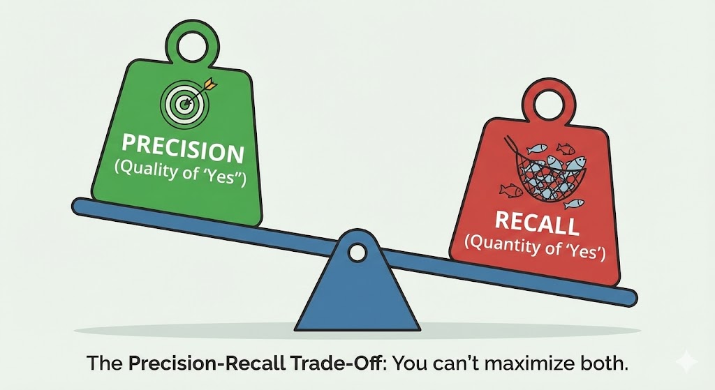
4.4: The Precision-Recall Trade-Off
Here is the uncomfortable truth: Precision and Recall are in tension.
Imagine a slider. On the left end, the model is extremely cautious—it only says “Cancer” when it is 99% sure. This gives you high Precision (its predictions are trustworthy) but low Recall (it misses many borderline cases).
On the right end, the model is extremely aggressive—it flags anything even slightly suspicious as “Cancer.” This gives you high Recall (it catches everything) but low Precision (most of its alarms are false).
The slider is the classification threshold. Most classifiers don’t just output “Cancer” or “Not Cancer.” They output a probability, like $0.73$ (73% chance of cancer). You then decide: “I will classify anything above $0.5$ as cancer.”
- Raise the threshold to $0.9$: Only very confident predictions count as positive. Precision goes up, Recall goes down.
- Lower the threshold to $0.2$: Even vaguely suspicious cases get flagged. Recall goes up, Precision goes down.
There is no universally “correct” threshold. The right choice depends entirely on the cost of each type of error in your specific domain.
4.5: F1-Score — The Peacemaker
What if you want a single number that balances both Precision and Recall? That is the F1-Score.
$$F1 = 2 \times \frac{Precision \times Recall}{Precision + Recall}$$
$$F1 = 2 \times \frac{0.727 \times 0.80}{0.727 + 0.80} = 2 \times \frac{0.582}{1.527} = 0.762$$
What it means: The F1-Score is the harmonic mean of Precision and Recall. It punishes extreme values. If either Precision or Recall is very low, the F1-Score will be dragged down, even if the other is high.
Why harmonic mean instead of arithmetic mean?
If you used a simple average: a model with $Precision = 1.0$ and $Recall = 0.0$ would get a score of $0.5$—which sounds “okay.” But a model with $0%$ recall has caught zero positive cases. It is useless. The harmonic mean would give this same model an F1 of $0.0$, correctly reflecting that it is broken.
When to use F1:
- When you need a single metric to compare models and you care about both Precision and Recall roughly equally.
- When the dataset is imbalanced and accuracy is unreliable.
Variants:
- F0.5-Score: Weighs Precision more heavily (useful in spam filters).
- F2-Score: Weighs Recall more heavily (useful in medical screening).
4.6: Specificity — The Forgotten Metric
$$Specificity = \frac{TN}{TN + FP}$$
$$Specificity = \frac{870}{870 + 30} = \frac{870}{900} = 96.7%$$
What it means: Of all the patients who are truly healthy, how many did the model correctly identify as healthy?
Why it matters: In a medical context, Specificity tells you: “How good is this model at ruling OUT the disease?” A model with low specificity will send thousands of healthy people into unnecessary follow-up procedures, overwhelming the healthcare system.
While Recall (Sensitivity) asks “did you find all the sick people?”, Specificity asks “did you correctly leave the healthy people alone?”
5: Beyond Binary — The AUC-ROC Curve
So far, we have been picking a single threshold and evaluating the model at that one point. But what if we could evaluate the model across all possible thresholds simultaneously?
This is the ROC Curve (Receiver Operating Characteristic).
How It Works
- Start with a threshold of $1.0$ (the model says “Cancer” for nothing). Plot the point.
- Lower the threshold slightly (e.g., $0.95$). More cases get flagged as positive. Plot the new True Positive Rate (Recall) vs. False Positive Rate ($1 - Specificity$).
- Keep lowering the threshold until it hits $0.0$ (the model says “Cancer” for everything).
- Connect all the dots. You get a curve.
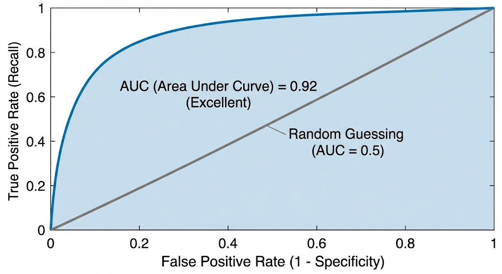
Reading the Curve
- The X-axis is the False Positive Rate (FPR). How many healthy people are you wrongly alarming?
- The Y-axis is the True Positive Rate (TPR / Recall). How many sick people are you catching?
- The diagonal line from $(0,0)$ to $(1,1)$ represents a model that is purely guessing (flipping a coin).
A good model’s curve will bow towards the upper-left corner, meaning it achieves high Recall without many False Positives.
The AUC (Area Under the Curve)
The AUC summarizes the entire ROC curve into a single number between $0$ and $1$.
| AUC Value | Interpretation |
|---|---|
| $1.0$ | Perfect model (exists only in textbooks) |
| $0.9 - 1.0$ | Excellent |
| $0.8 - 0.9$ | Good |
| $0.7 - 0.8$ | Fair |
| $0.5$ | Random guessing (coin flip) |
| $< 0.5$ | Worse than random (your labels might be flipped) |
Why AUC is powerful: It is threshold-independent. It tells you: “Across all possible operating points, how well does this model separate the two classes?” This makes it an excellent metric for comparing models before you’ve even decided on a threshold.
When to use AUC-ROC:
- When you want to compare models in a threshold-agnostic way.
- When you need to present model performance to stakeholders who don’t understand the Precision-Recall trade-off.
- When you are working on ranking problems (e.g., “rank these emails from most likely spam to least likely spam”).
6: Regression Metrics — When the Answer Is a Number
Not every AI model classifies things into categories. Many models predict continuous numbers: the price of a house, the temperature tomorrow, the revenue next quarter. These are Regression models, and they need their own set of metrics.
6.1: Mean Absolute Error (MAE)
$$MAE = \frac{1}{n} \sum_{i=1}^{n} |y_i - \hat{y}_i|$$
What it means: On average, how far off are the model’s predictions from the actual values?
Example: If a house price predictor has an MAE of $$25,000$, it means on average, the model’s prediction is $$25,000$ away from the true price—sometimes above, sometimes below.
Strength: Easy to interpret. Treats all errors equally. A $$10,000$ error is twice as bad as a $$5,000$ error—no more, no less.
6.2: Mean Squared Error (MSE) and Root Mean Squared Error (RMSE)
$$MSE = \frac{1}{n} \sum_{i=1}^{n} (y_i - \hat{y}_i)^2$$
$$RMSE = \sqrt{MSE}$$
What it means: Similar to MAE, but it squares the errors before averaging them. This means large errors are penalized disproportionately.
Why it matters: If your house price model is off by $$5,000$ on most houses but off by $$500,000$ on one mansion, the MAE might still look reasonable. But the MSE will explode, because $(500,000)^2$ is enormous. MSE screams: “You have a catastrophic outlier prediction!”
When to use which:
- MAE when you want a robust, interpretable metric that doesn’t overreact to outliers.
- RMSE when large errors are particularly unacceptable (e.g., medical dosage predictions, where being off by a large amount could be fatal).
6.3: R-Squared ($R^2$) — The Explained Variance
$$R^2 = 1 - \frac{\sum (y_i - \hat{y}_i)^2}{\sum (y_i - \bar{y})^2}$$
What it means: How much of the variance in the data does the model explain? It compares your model to a “dumb baseline” that always predicts the average value.
| $R^2$ Value | Interpretation |
|---|---|
| $1.0$ | The model perfectly explains all variance |
| $0.8$ | The model explains 80% of the variance |
| $0.0$ | The model is no better than predicting the mean |
| Negative | The model is worse than predicting the mean |
The key insight: $R^2$ tells you whether your model has learned any signal at all. A negative $R^2$ means you would literally be better off ignoring the model and just guessing the average every time.
7: The Language Model Problem — How Do You Evaluate Words?
Everything we have discussed so far works for structured problems: classify an image, predict a number. But what about the models dominating the headlines today—Large Language Models (LLMs) like GPT-4, Claude, Gemini, and Llama?
How do you evaluate whether a model has written a “good” essay? A “correct” summary? A “helpful” response?
This is one of the hardest open problems in AI. There is no confusion matrix for creativity. There is no F1-Score for helpfulness.
But we have made significant progress. Let’s walk through the key evaluation approaches.
7.1: Perplexity — “How Surprised Is the Model?”
Perplexity is the classic metric for language models. It predates the LLM era and comes from information theory.
$$Perplexity = 2^{H(p)}$$
where $H(p)$ is the cross-entropy of the model’s predictions against the actual next tokens.
Intuition: Imagine you are reading a sentence: “The cat sat on the ____.”
A good language model should predict the next word is probably “mat,” “floor,” “couch,” or “table.” It should not be surprised by these words. It should assign them high probability.
If the actual next word is “mat” and the model had already assigned a high probability to “mat,” the model has low perplexity. It wasn’t surprised.
If the actual next word is “mat” but the model thought the next word was going to be “supernova,” the model has high perplexity. It was very confused.
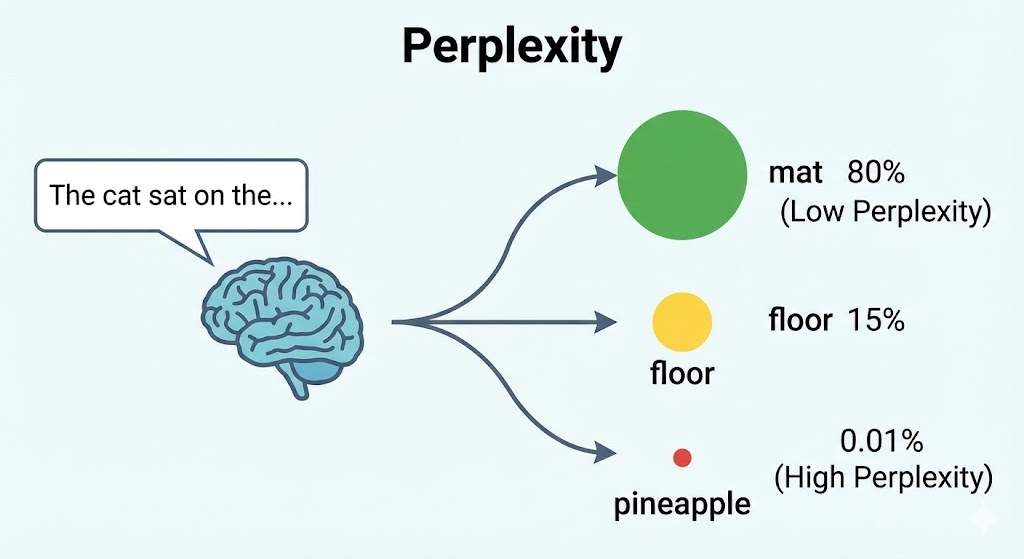
Lower perplexity = better model. A perplexity of $1$ would mean the model perfectly predicted every next word with 100% confidence.
| Perplexity | Interpretation |
|---|---|
| ~$1$ | Impossibly perfect prediction |
| ~$20-50$ | Very good (modern LLMs on standard benchmarks) |
| ~$100-200$ | Mediocre |
| ~$1000+$ | The model is essentially guessing randomly |
Limitation: Perplexity only measures how well the model predicts the next token. It says nothing about whether the generated text is useful, truthful, coherent, or safe. A model could have excellent perplexity and still confidently generate harmful misinformation.
7.2: BLEU Score — Evaluating Translations and Summaries
The BLEU Score (Bilingual Evaluation Understudy) was designed for machine translation but is widely used for any text generation task where you have a reference answer.
How it works: It compares the model’s output to one or more “reference” translations (human-written gold standards) and counts how many word sequences (n-grams) overlap.
Example:
- Reference: “The cat is sitting on the mat.”
- Model Output A: “The cat is on the mat.” (Pretty close!)
- Model Output B: “A feline rests upon a floor covering.” (Semantically similar, but very different words.)
BLEU would score Output A much higher than Output B because it shares more exact n-grams with the reference, even though Output B might actually be a perfectly valid translation.
| BLEU Score | Interpretation |
|---|---|
| $> 0.6$ | Very high quality (close to human translation) |
| $0.4 - 0.6$ | Good, understandable |
| $0.2 - 0.4$ | The gist is right, but rough around the edges |
| $< 0.2$ | Poor quality |
Limitations of BLEU:
- It is purely lexical. It counts word overlaps. It does not understand meaning.
- “The cat sat on the mat” and “A feline rested upon the rug” have the same meaning but almost zero n-gram overlap. BLEU would score the second one poorly.
- It penalizes creative or paraphrased outputs, even when they are perfectly valid.
This is why BLEU is increasingly seen as insufficient for evaluating modern generative AI. A model that simply copies the reference verbatim would score perfectly.
7.3: ROUGE — The Recall-Oriented Alternative
ROUGE (Recall-Oriented Understudy for Gisting Evaluation) is the counterpart to BLEU, primarily used for evaluating text summarization.
Where BLEU focuses on Precision (how much of the model’s output matches the reference), ROUGE focuses on Recall (how much of the reference is captured in the model’s output).
- ROUGE-1: Overlap of unigrams (individual words).
- ROUGE-2: Overlap of bigrams (two-word sequences).
- ROUGE-L: Longest Common Subsequence between the output and reference.
When to use ROUGE: When you care that the summary covers all the important points from the original text, not just that it uses the exact same words.
7.4: The Human Evaluation Frontier
Here is the uncomfortable truth: for modern LLMs, automated metrics are often inadequate.
A model can have low perplexity, reasonable BLEU scores, and still produce outputs that are:
- Factually wrong (hallucinations)
- Subtly biased
- Logically incoherent across paragraphs
- Technically correct but unhelpful
- Safe but utterly boring
This is why the frontier of LLM evaluation is increasingly turning to human judgment and model-as-judge approaches.
Human Evaluation Dimensions
When human evaluators assess LLM outputs, they typically score along multiple dimensions:
| Dimension | What It Measures |
|---|---|
| Helpfulness | Did the response actually answer the question? Was it useful? |
| Truthfulness | Are the facts correct? Are citations real? |
| Harmlessness | Does the response avoid generating dangerous, biased, or offensive content? |
| Coherence | Does the response flow logically? Is it well-structured? |
| Relevance | Does the response stay on topic? |
| Conciseness | Does it answer efficiently without unnecessary padding? |
The ELO Rating System (Chatbot Arena)
One of the most influential evaluation methods for LLMs today is the Chatbot Arena, developed by researchers at UC Berkeley (LMSYS). It works like a chess rating system:
- A human user submits a prompt.
- Two anonymous LLMs generate responses side by side.
- The human picks which response is better (or declares a tie).
- Both models get an ELO rating update based on the result.
Over thousands of battles, a leaderboard emerges. This approach is powerful because it captures the holistic quality of a response—something no automated metric can fully do.
LLM-as-Judge
A newer approach uses a powerful LLM (like GPT-4 or Claude) to evaluate the outputs of other models. You give the “judge” model a rubric:
“Rate the following response on a scale of 1-5 for helpfulness, accuracy, and safety. Explain your reasoning.”
This is faster and cheaper than human evaluation, and studies have shown it correlates surprisingly well with human judgments for many tasks.
The catch: The judge model has its own biases. It may prefer verbose responses, or responses written in its own style. It may confidently rate a factually wrong answer as “correct” if the answer is well-written.
8: The Benchmark Wars — Standardized Tests for AI
Just like SAT scores let universities compare applicants, the AI field has developed standardized benchmarks to compare models. Here are the most important ones:
For Language Models
| Benchmark | What It Tests |
|---|---|
| MMLU (Massive Multitask Language Understanding) | 57 subjects from STEM to law to history. Tests broad knowledge. |
| HumanEval | Can the model write working Python code from a docstring? |
| GSM8K | Grade-school math word problems. Tests mathematical reasoning. |
| TruthfulQA | Does the model resist generating common misconceptions? |
| HellaSwag | Commonsense reasoning (predict what happens next in a scenario). |
| ARC (AI2 Reasoning Challenge) | Science questions that require reasoning, not just retrieval. |
| MT-Bench | Multi-turn conversation quality, judged by GPT-4. |
The Problem with Benchmarks
Benchmarks have a fundamental weakness: Goodhart’s Law.
“When a measure becomes a target, it ceases to be a good measure.”
Once a benchmark becomes popular, model developers begin optimizing specifically for it. They might:
- Train on data that is suspiciously similar to the benchmark questions.
- Use techniques that boost benchmark scores without improving real-world capability.
- Cherry-pick which benchmarks to report (showing only the ones where their model excels).
This phenomenon is called benchmark contamination or benchmark gaming, and it is increasingly recognized as a serious problem in AI evaluation. A model might score 90% on MMLU but fail spectacularly at a simple real-world task that wasn’t covered by the benchmark.
Quote
Benchmarks are like standardized tests for students. They measure something real, but they do not measure everything that matters. The student who aces the SAT might still struggle with a job interview.
9: The Emerging Frontier — Evaluating What Matters Most
As AI systems become more powerful and more embedded in critical decisions, the evaluation criteria are expanding far beyond accuracy.
9.1: Fairness and Bias
A model can be “accurate” on average while being systematically unfair to specific groups. A hiring algorithm might achieve 90% overall accuracy but reject qualified female candidates at twice the rate of male candidates.
Key fairness metrics include:
- Demographic Parity: Does the model approve roughly equal proportions of candidates across protected groups?
- Equalized Odds: Does the model have equal True Positive and False Positive rates across groups?
- Calibration: If the model says a candidate has an 80% chance of being qualified, is that true for all demographic groups, or only some?
9.2: Robustness
How does the model behave when the input is slightly unusual?
A self-driving car model trained in sunny California might fail catastrophically in a snowstorm in Minnesota. An NLP model trained on formal English might break when given slang, typos, or a different dialect.
Robustness testing involves:
- Adversarial attacks: Intentionally crafting inputs designed to fool the model (e.g., adding imperceptible noise to an image that causes it to be misclassified).
- Distribution shift: Testing the model on data that is statistically different from the training data.
- Edge cases: Testing on rare, unusual, or extreme inputs.
9.3: Calibration
A model is well-calibrated if its confidence scores are meaningful.
If the model says “I am 90% confident this is a cat,” then across all cases where it says “90% confident,” it should actually be correct about 90% of the time.
Many modern neural networks are overconfident—they output high probability scores even when they are wrong. A poorly calibrated model that says “99% sure” and is wrong 30% of the time is dangerous, because humans trust the confidence score and make high-stakes decisions based on it.
9.4: Latency and Efficiency
In production, a model that takes 30 seconds to respond is useless for a real-time application, even if it has perfect accuracy. Evaluation increasingly includes:
- Inference latency: How fast does the model respond?
- Throughput: How many requests can it handle per second?
- Model size: Can it run on edge devices (phones, IoT sensors)?
- Energy consumption: What is the environmental cost per prediction?
A smaller model that achieves 92% accuracy in 10 milliseconds is often more “good” than a massive model that achieves 95% accuracy in 5 seconds—depending on the use case.
9.5: Explainability
Can the model explain why it made a decision?
In many regulated industries (healthcare, finance, criminal justice), a black-box prediction is unacceptable, regardless of accuracy. Regulators and patients need to understand why the model denied a loan, recommended a treatment, or flagged a transaction.
This is the domain of Explainable AI (XAI), which includes techniques like:
- SHAP (SHapley Additive exPlanations): Assigns importance scores to each input feature.
- LIME (Local Interpretable Model-Agnostic Explanations): Builds a simple, interpretable model around a single prediction.
- Attention Visualization: In Transformer models, visualizing which parts of the input the model “paid attention to.”
A model that is 93% accurate and fully explainable may be far more “good” than a model that is 97% accurate but a complete black box.
10: The Python Practitioner’s Toolkit
Let’s ground all of this theory in code. Here is how you would compute the key metrics in Python using scikit-learn.
from sklearn.metrics import (
    accuracy_score,
    precision_score,
    recall_score,
    f1_score,
    confusion_matrix,
    classification_report,
    roc_auc_score,
    roc_curve,
    mean_absolute_error,
    mean_squared_error,
    r2_score,
)
import numpy as np

# --- CLASSIFICATION EXAMPLE ---
# Simulated ground truth labels and model predictions
# 1 = Cancer, 0 = Not Cancer
y_true = [1, 1, 1, 1, 1, 0, 0, 0, 0, 0, 0, 0, 0, 0, 0, 1, 1, 1, 0, 0]
y_pred = [1, 1, 1, 0, 1, 0, 0, 1, 0, 0, 0, 0, 0, 0, 0, 1, 0, 1, 0, 0]

# --- ACCURACY ---
acc = accuracy_score(y_true, y_pred)
print(f"Accuracy: {acc:.2%}")
# Output: Accuracy: 85.00%

# --- PRECISION ---
prec = precision_score(y_true, y_pred)
print(f"Precision: {prec:.2%}")
# Output: Precision: 85.71%

# --- RECALL ---
rec = recall_score(y_true, y_pred)
print(f"Recall: {rec:.2%}")
# Output: Recall: 75.00%

# --- F1 SCORE ---
f1 = f1_score(y_true, y_pred)
print(f"F1-Score: {f1:.2%}")
# Output: F1-Score: 80.00%

# --- CONFUSION MATRIX ---
cm = confusion_matrix(y_true, y_pred)
print(f"\nConfusion Matrix:\n{cm}")
# Output:
# [[11  1]
#  [ 2  6]]

# --- FULL CLASSIFICATION REPORT ---
print("\nFull Classification Report:")
print(classification_report(y_true, y_pred, target_names=["Healthy", "Cancer"]))

# --- AUC-ROC ---
# For AUC, we need probability scores, not just hard predictions.
# Simulated probability scores from the model:
y_prob = [0.9, 0.8, 0.7, 0.4, 0.85, 0.1, 0.2, 0.6, 0.15, 0.05,
          0.1, 0.2, 0.3, 0.1, 0.05, 0.75, 0.35, 0.88, 0.12, 0.08]

auc = roc_auc_score(y_true, y_prob)
print(f"\nAUC-ROC Score: {auc:.4f}")
# A score close to 1.0 indicates excellent class separation.
# --- REGRESSION EXAMPLE ---
# Simulated: Actual house prices vs. model's predicted prices (in $1000s)
y_true_reg = [300, 450, 200, 520, 380, 410, 275, 600, 350, 490]
y_pred_reg = [310, 430, 220, 500, 370, 425, 260, 580, 365, 475]

# --- MAE ---
mae = mean_absolute_error(y_true_reg, y_pred_reg)
print(f"MAE: ${mae:.2f}k")
# Output: MAE: $17.00k (On average, the model is off by $17,000)

# --- RMSE ---
mse = mean_squared_error(y_true_reg, y_pred_reg)
rmse = np.sqrt(mse)
print(f"RMSE: ${rmse:.2f}k")
# Output: RMSE: $18.17k

# --- R-Squared ---
r2 = r2_score(y_true_reg, y_pred_reg)
print(f"R² Score: {r2:.4f}")
# Output: R² Score: 0.9786 (The model explains ~97.8% of the variance. Excellent!)
11: A Decision Framework — Choosing the Right Metric
After all of this, the natural question is: “Okay, so which metric should I use?”
There is no universal answer. But here is a framework to guide your decision:
Step 1: What type of problem are you solving?
- Binary Classification (Yes/No) → Precision, Recall, F1, AUC-ROC
- Multi-Class Classification (Cat/Dog/Bird) → Macro/Micro/Weighted F1, Confusion Matrix
- Regression (Predict a number) → MAE, RMSE, R²
- Text Generation → Perplexity, BLEU, ROUGE, Human Evaluation
- Ranking (Search results, recommendations) → NDCG, MAP, MRR
Step 2: What is the cost of each type of error?
- False Negatives are expensive (missed cancer, missed fraud) → Optimize for Recall
- False Positives are expensive (blocked emails, false accusations) → Optimize for Precision
- Both are equally bad → Optimize for F1-Score
Step 3: Is your dataset imbalanced?
- Yes (rare disease, fraud) → Do NOT use accuracy. Use F1, AUC-ROC, or Precision-Recall AUC.
- No (balanced classes) → Accuracy is a reasonable starting point, supplemented by F1.
Step 4: Do you need to explain the model’s decisions?
- Yes (healthcare, finance, legal) → Add explainability metrics (SHAP, LIME). Consider simpler, interpretable models.
- No (image filters, game AI) → Focus on performance metrics.
Step 5: What are the production constraints?
- Real-time application → Latency and throughput matter as much as accuracy.
- Edge deployment → Model size and efficiency are critical.
- High-trust domain → Calibration and uncertainty estimation are essential.
12: Conclusion — The Metric Is the Mission
Here is the most important takeaway from this entire article:
The metric you choose defines what your model learns to care about.
If you optimize for accuracy on an imbalanced dataset, your model learns to be lazy—predicting the majority class every time and ignoring the minority cases that matter most.
If you optimize for Recall in a spam filter, your model learns to be paranoid—flagging everything, including your boss’s emails.
If you optimize for BLEU in a translation system, your model learns to parrot the reference text verbatim instead of generating natural, fluent translations.
The choice of metric is not a technical afterthought. It is a design decision. It reflects your values, your priorities, and your understanding of the problem domain. It is, in a very real sense, the soul of your AI system.
A truly “good” AI is not the one with the highest number on a leaderboard. It is the one that makes the right kind of mistakes for its specific context. It is the one where the engineers sat down, thought carefully about the consequences of each type of error, and chose to optimize for the metric that minimizes real-world harm.
So the next time someone shows you a model and says, “It’s 97% accurate!"—ask them:
“97% accurate at what? Measured how? On whose data? And what happens when it’s wrong?”
Because in AI, how you measure “good” is the most important decision you will ever make.

